How to Create a Flower Pattern in Microsoft Excel

The Tutorial

1. In the previous article, How to Create Artistic Patterns in Microsoft Excel, a Data worksheet was described in great detail. This will be a continuation from that article, so please complete that one first.
2. How to Create a Flower Pattern in Microsoft Excel Picture 1
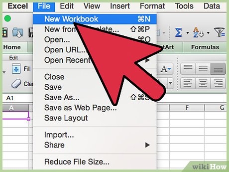
   Start a new workbook by saving the old workbook under a new name.
3. How to Create a Flower Pattern in Microsoft Excel Picture 2
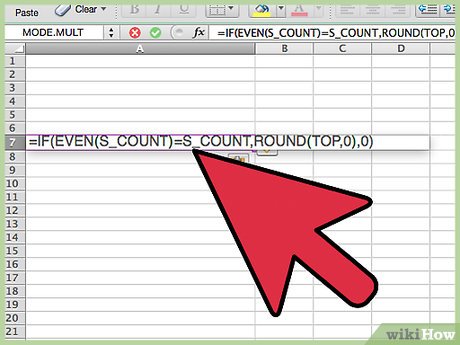
   The defined variable "top" is being moved and its formula is being changed, to start with. Please copy cell A7 to cell C3. Make sure that cell C3 has the Defined Variable Name top. Change the formula in A7 to "=IF(EVEN(S_COUNT)=S_COUNT,ROUND(TOP,0),0)". Select both cells A7 and C3 using the Command Key and Format (both) Cells Fill Purple, Border Red bold Outline, Font bold, Align horizontal center, Number Number  Decimal Places 4. The formula in cell C3 should be "=ROUND((-A4*PI())+(Adj),0)" and the result should be 968133.0000 (for now).
4. How to Create a Flower Pattern in Microsoft Excel Picture 3
   The notes in cells E3:E5 have changed a bit;

   1. E3: Put "Y" for Spheres / Spheroids proportionally, whether even/odd S_COUNT (in B1)
   2. E4:  For S_COUNT (B1) > 25, overlapping = "Y" input, otherwise input "N"
   3. E5: Also: "N" input results in full circle of spheroids / podoids whether odd or even. 
5. How to Create a Flower Pattern in Microsoft Excel Picture 4
   Edit Go To cell range D7:D1447 and with D7 active input w/o quotes the formula "=SIN((ROW()-7)*Factor*PI()/180)" and Edit Fill Down. (It's no longer squared).
6. How to Create a Flower Pattern in Microsoft Excel Picture 5
   Edit Go To cell range E7:E1447 and input w/o quotes the formula "=(PI())*((SIN(A7/(B7*2))*1*COS(A7)*1*(COS(A7/(B7*2)))*1)+C7)*SIN(A7/(B7*2))" and Edit Fill Down.
7. How to Create a Flower Pattern in Microsoft Excel Picture 6
   Edit Go To cell range F7:F1447 and input w/o quotes the formula "=(PI())*((SIN(A7/(B7*2))*1*SIN(A7)*1*(COS(A7/(B7*2)))*1)+D7)*SIN(A7/(B7*2))" and Edit Fill Down.
8. How to Create a Flower Pattern in Microsoft Excel Picture 7
   Select cell A5 and enter w/o quotes the formula "=IF(TURNS>0,VLOOKUP(TURNS,TURNS_LOOKUP,2),VLOOKUP(TURNS, TURNS_LOOKUP_NEG,2))". This will result in a #NAME error which will soon be gone.
9. How to Create a Flower Pattern in Microsoft Excel Picture 8
   Cell L1 should read TURNS_LOOKUP, else enter it.

   1. Select cell range L2:L1441 and input 1 and then do Edit Fill Series Columns Linear Step Value 1 OK.
   2. Enter 72 into cell M1 and -440 into cell M2 and select cell range M2:M1441 and do Edit Fill Series Column Linear Step Value 72, OK.
   3. Select cell range L2:M1441 and Insert Name Define TURNS_LOOKUP to cell range $L$2:$M$1441 and Format Cells Border Blue bold Outline.
10. How to Create a Flower Pattern in Microsoft Excel Picture 9
    Select cell O1 and enter TURNS_LOOKUP_NEG.

    1. Edit Go To cell range O2:O1442 and enter -1440 and do Edit Fill Series Column Linear Step Value 1, OK.
    2. Edit select cell P1442 and enter the formula "=M2-$M$1".
    3. Go To cell P1441 and enter the formula w/o quotes "=P1442-$M$1" and copy that cell and paste it to cell range P1440:P2.
    4. Edit Go To cell range O2:P1442 and Insert Name Define Name TURNS_LOOKUP_NEG to cell range $O$2:$P$1442 and Format Cells Border Red bold Outline.
11. How to Create a Flower Pattern in Microsoft Excel Picture 10
    Copy from the following pictures the cell range R1:S1441. sometimes manually, sometimes automatically, per the differences column appearing in column T at right: and continue at 300 rate until the end, and then do:

    1. Edit Go To cell range R2:S1441 and Insert Name Define name SPHEROIDS_COUNT_LOOKER to cell range $R$2:$S$1441 and Format Cells Border Red bold Outline.
12. How to Create a Flower Pattern in Microsoft Excel Picture 11
    Select cell B2 and enter the formula w/o quotes "=VLOOKUP(S_COUNT,SPHEROIDS_COUNT_LOOKER,2)".
13. How to Create a Flower Pattern in Microsoft Excel Picture 12
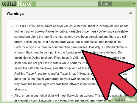
    Look for errors and correct any that appear. See Warnings section below on how to go about doing so if having trouble.

Explanatory Charts, Diagrams, Photos

1. (dependent upon the tutorial data above)

1. How to Create a Flower Pattern in Microsoft Excel Picture 13
   Create the Chart.

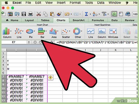
   1. Select cell range E7:F1446 and do Chart Wizard and follow along or choose Charts on the Ribbon and select All/Other and scroll down to Scatter, Smoothed Line Scatter, and a new small chart should appear atop your data. Copy or Cut and Paste it to the Chart worksheet cell A1 and hover over the lower right corner until the cursor becomes a double-headed arrow then click and expand it it open. Do Chart Layout Format Selection at far left and choose Series 1, Line Weight 1, Color Blueish Purple, and then click on the Plot Area and Format Selection Fill Solid Black. Select series G7:H1446 and I7:J1446 and copy and paste those into the chart and correct the data series and get rid of any extra straight lines that appear. The correct series appear below. Select the on the Data sheet I7:J1446 and make the Line Weight 1 and color Ice Blue. Select the on the Data sheet G7:H1446 and make the Line Weight 1 and color Reddish Brown. Then change the series order of how the three series display until you have it so that
   2. =SERIES(,Data!$G$7:$G$1446,Data!$H$7:$H$1446,1) is Series 1 via the 1 at the very end of the series description;
   3. =SERIES(,Data!$I$7:$I$1446,Data!$J$7:$J$1446,2) is Series 2;
   4. =SERIES(,Data!$E$7:$E$1446,Data!$F$7:$F$1446,3) is Series 3.
2. How to Create a Flower Pattern in Microsoft Excel Picture 14
   Holding the shift key down, Copy Picture and activate the Saves worksheet and Paste Picture. Save the Workbook and you're done!

   1. How to Create a Flower Pattern in Microsoft Excel Picture 15

      SPCL DESIGN 02

Helpful Guidance

1. Make use of helper articles when proceeding through this tutorial:

   1. See the article How to Create a Spirallic Spin Particle Path or Necklace Form or Spherical Border for a list of articles related to Excel, Geometric and/or Trigonometric Art, Charting/Diagramming and Algebraic Formulation.
   2. For more art charts and graphs, you might also want to click on Category:Microsoft Excel Imagery, Category:Mathematics, Category:Spreadsheets or Category:Graphics to view many Excel worksheets and charts where Trigonometry, Geometry and Calculus have been turned into Art, or simply click on the category as appears in the upper right white portion of this page, or at the bottom left of the page.