How to Use the TRUNC Function in Excel

The Excel TRUNC function removes digits from a number without rounding. You can keep a specified number of decimal places, return the integer portion, or truncate positions to the left of the decimal point.

Syntax

=TRUNC(number, [num_digits])

• number: the value to truncate.
• num_digits: the number of decimal places to keep. It is optional and defaults to 0.

For example, =TRUNC(4.68) returns 4, while =TRUNC(4.68,1) returns 4.6. Unlike ROUND, TRUNC simply discards digits.

Remove the decimal portion

With a value in A2, use:

=TRUNC(A2)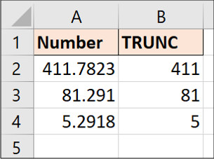

If A2 contains 411.98, the result is 411. For negative numbers, TRUNC moves toward zero: =TRUNC(-4.68) returns -4. This differs from INT(-4.68), which returns -5.

Keep a selected number of decimal places

To keep two decimal places:

=TRUNC(A2,2)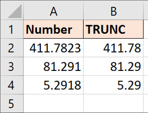

If the source has fewer than two decimal places, its numeric value does not change.

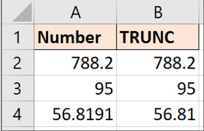
TRUNC does not add trailing zeros for display. To show a fixed number of decimal places, apply a number format to the result cell.

Remove the time from a date-time value

Excel stores a date as the integer portion of a serial number and time as the fractional portion. If A2 contains a valid Excel date and time, this formula removes the time:

=TRUNC(A2)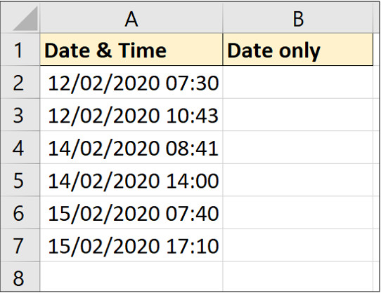

Format the result as a date.

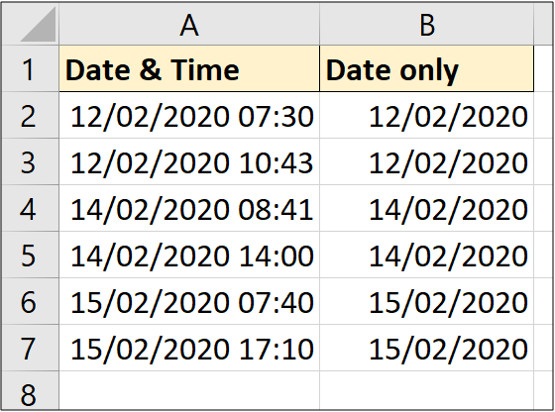
If the source is text rather than a real Excel date-time value, convert it before using TRUNC.

Truncate digits to the left of the decimal point

A negative num_digits replaces positions to the left of the decimal point with zeros:

=TRUNC(A2,-1)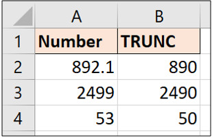

For 487.25, this returns 480. With -2, it returns 400. The result is truncation, not rounding.

TRUNC, ROUND, and INT

Use TRUNC when discarded digits must not affect the result. To compare nearly equal values before matching, see how to match data in Excel. For a broader reference, review the Excel statistical functions guide.