Gradient Descent for Linear Regression: A JavaScript Example

Gradient descent trains a linear regression model by repeatedly adjusting its slope and intercept to reduce prediction error. This example fits a line ŷ = wx + b to paired x and y values, then measures how far its predictions are from the observations.

What changes during training

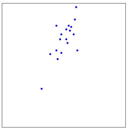
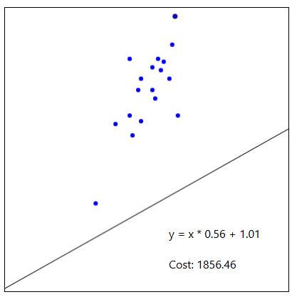
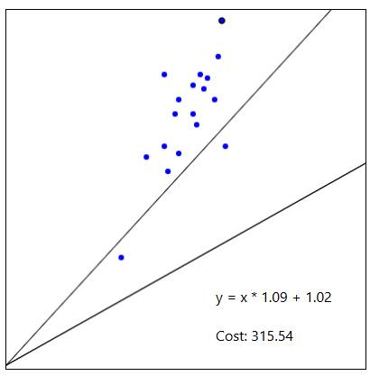
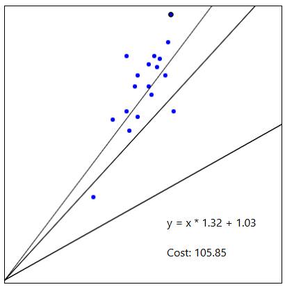
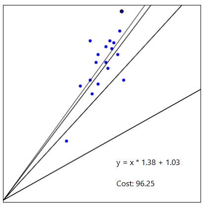
The weight w controls the line's slope and the bias b controls its intercept. For each point, the residual is (wx + b) − y. Mean squared error (MSE) averages the squares of those residuals over all N points. Squaring makes large misses count more and gives this model a smooth objective to minimize. If you are new to the model, see our linear regression introduction.

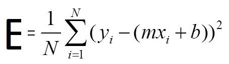
In symbols, MSE = (1/N) Σ(wxᵢ + b − yᵢ)². A training step computes the loss gradient for both parameters and subtracts a small multiple of it. The learning rate controls that step size; there is no universally correct fixed value.

A complete JavaScript example

The following implementation keeps the error sum local and uses a small dataset. Run it in a browser console or Node.js:

function trainLine(xs, ys, rate = 0.01, epochs = 1000) {
  if (xs.length !== ys.length || xs.length === 0) {
    throw new Error('Provide matching nonempty x and y arrays');
  }
  let weight = 0;
  let bias = 0;
  const n = xs.length;

  for (let epoch = 0; epoch < epochs; epoch++) {
    let weightGradient = 0;
    let biasGradient = 0;
    for (let i = 0; i < n; i++) {
      const error = weight * xs[i] + bias - ys[i];
      weightGradient += (2 * error * xs[i]) / n;
      biasGradient += (2 * error) / n;
    }
    weight -= rate * weightGradient;
    bias -= rate * biasGradient;
  }

  const mse = xs.reduce((sum, x, i) => {
    const error = weight * x + bias - ys[i];
    return sum + error * error;
  }, 0) / n;
  return { weight, bias, mse };
}

const model = trainLine([0, 1, 2, 3, 4], [1, 3, 5, 7, 9]);
console.log(model); // weight approaches 2, bias approaches 1
console.log(model.weight * 5 + model.bias); // prediction near 11

The example uses full-batch gradient descent: each update sums the gradient from every observation. The parameters are updated after the inner loop, so both gradients refer to the same line. For this simple linear pattern, the fitted line should approach y = 2x + 1.

Diagnose the learning curve

Log MSE at intervals to check whether it generally declines. If it rises or becomes NaN, inspect the input arrays and try a smaller learning rate; very large feature values can make a previously reasonable step size unstable. If it decreases extremely slowly, adjust the rate or scale the features. Fixed training iterations do not prove a model is ready: compare its predictions on data withheld from training and with a simple baseline. Google's gradient descent explanation provides the mathematical picture, and our machine learning fundamentals course covers evaluation.