How to Make Your Excel Curve Solid or Transparent
In this article, you'll learn to make your curves, in this case the Garthwaite Curves, solid or transparent and surround them in a realistic modern frame. Become familiar with the image to create: === The tutorial ===
Table of Contents
Part 1 of 3:
The tutorial
-
 Open a new workbook and save it under an appropriate title for this project. Create 3 worksheets: Data, Chart (unless working with Chart Wizard) and Saves.
 -
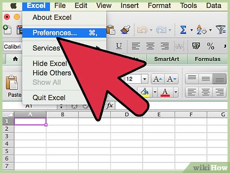 Set the Preferences under the Excel menu:
- In General, set R1C1 to Off and select Show the 10 Most Recent Documents .
- In Edit, set all the first options to checked except Automatically Convert Date System . Set Display number of decimal places to blank (as integers are preferred). Preserve the display of dates and set 30 for 21st century cutoff.
- In View, click on show Formula Bar and Status Bar and hover for comments of all Objects . Check Show grid lines and set all boxes below that to auto or checked.
- In Chart, allow show chart names and set data markers on hover and leave the rest unchecked for now.
- In Calculation, make sure Automatically is checked and calculate before save is also checked. Set max change to .001 as goal-seeking is not done in this project. Check save external link values and use 1904 system
- In Error checking, check all the options.
- In Save, select save preview picture with new files and Save Autorecover after five minutes
- In Ribbon, keep all of them checked except Hide group titles and Developer .
-
 Go to cell A29 and do Freeze Panes under the Window menu. It helps by placing the cursor between the A of Column A and the 1 in Row 1 in the upper leftmost corner and selecting the entire worksheet. Format Cells Number Number Custom +0.00;-0.00;+0.00, Font Size 9 or 10.
 -
 Create the Defined Variables Upper Section (here's a picture):
- Into cell A1 enter ADJROWS and into cell B1 enter 2880.
- Into cell C1 enter SPHEROIDS and into cell D1 enter 36.
- Into cell E1 enter BASE and into cell F1 enter "=16*103*24/(SPHEROIDS*2)" w/o quotes.
- Into cell A2 enter Rrs and into cell B2 enter "=ADJROWS/SPHEROIDS" w/o quotes.
- Into cell C2 enter Radius and into cell D2 enter "=SPHEROIDS/VLOOKUP(SPHEROIDS,LOOKER3,2)" w/o quotes.
- Into cell E2 enter FACTOR and into cell F2 enter "=VLOOKUP(SPHEROIDS,FactorLooker,3)" w/o quotes.
- Into cell A3 enter On_0_Off_1 and into cell B3 enter 0.
- Into cell C3 enter CircleFactor and into cell D3 enter 0.125 and format cell number number Custom +0.000;-0.000;+0.000
- Select cell range A1:B3 and Insert Name Create Names in Left Column, OK. Select cell range C1:D3 and Insert Name Create Names in Left Column, OK. Select cell range E1:F2 and Insert Name Create Names in Left Column, OK. There should not be anymore NAME errors except in D2 and F2 related to the Lookup Tables yet to be input.
- Format cells align right cell range I1:I3. Input to cell I1 SPHEROIDS2 and enter to J1 1.
- Into cell I2 enter BASE2 and into cell J2 enter "=16*103*24/(SPHEROIDS2*2)" w/o quotes.
- Into cell I3 enter ShrinkExpand and into J3 enter .75; select cell range I1:J3 and Insert Name Create Names in Left Column, OK.
- Into cell L1 enter FACTOR2 and into cell K1 enter 1.75. Into cell M1 make the note (formula overwritten).
- Into cell L2 enter Radius2 and into cell K2 enter "=SPHEROIDS2/VLOOKUP(SPHEROIDS2,LOOKER3,2)" w/o quotes.
- Into cell L3 enter ShrinkExpand2 and into cell K3 enter 2.
- Select cell range K1:L3 and Insert Name Create Names in Right Column, OK.
- Create the two Lookup Tables:
- Into cell L5 enter LOOKER3 and into cell N5 enter FactorLooker. Into cell L6 enter 1 and select range L6:L105 and Edit Fill Series Column Linear Step Value 1, OK. As for the rest of the top of the chart for cell range cell M1:N28, copy the values from the following picture please:

- For the values from M28:M105, they are all equal to 6. And all the values for cell range N28:N105 are equal to .8
- Edit Go To cell range L6:M105 and Insert Name Define Name LOOKER3 to cell range $L$6:$M$105.
- Edit Go To cell range L6:N105 and Insert Name Define Name FactorLooker to cell range $L$6:$N$105. Format fill cell range L6:N105 color canary yellow. Format cell N9 number number 6 decimal places (use the formula beside it to input it, w/o the leading period).
- Into cell L5 enter LOOKER3 and into cell N5 enter FactorLooker. Into cell L6 enter 1 and select range L6:L105 and Edit Fill Series Column Linear Step Value 1, OK. As for the rest of the top of the chart for cell range cell M1:N28, copy the values from the following picture please:
-
 Create the Column Headings:
- A4: Enter (1 ON 1 OFF). This means that every other spheroid will appear when the variable On_0_Off_1 is set to 0.
- A5: Enter OK to S=36. This means that the above On/Off mechanism works up to 36 spheroids. After that, the formula would have to be lengthened and there's a limit to how much further it can be lengthened.

- B4: Left2Right; B5: Top2Btm -- this means that by using 720 instead of ROW()-6 for the Cos and Sin calculations, the chart starts at the 12 o'clock position and moves clockwise left to right and top to bottom.
- C5: t; This is the traditional variable for the number of turns/spheroid but that's been changed.
- D5: Cos; E5: Sin
- F4, H4 and J4: Charting; G4: Solids; I4: Ring; K4: Center
- F5: Main X; G5: Main Y
- H5: X2; I5: Y2
- J5: X3; K5: Y3
-
 Format the Top Section:
- INPUT CELLS: Command+Select all the following cells: A3,D1,J1,K1 and K3. Format Fill yellow and font red bold size 14, with red border bold outline.
- Constants and Titles of the Solid (Main) Spheroids: Command+Select all of the following cells: B1,B2,D2,D3,F1,F2,F4 and G4. Format Fill black with white font size 12. Format cell D3 number number custom +0.000;-0.000;+0.000 (2880 rows * .125 = 360 degrees in a circle.).
- Constant and Title of the Spheroid Ring: Command+Select the following cells: H4,I4 and J3 and format fill dark/electric blue with white font, size 12.
- Variables, Constant and Titles of Center Spheroid: Command+Select the following cells C6,J2,K2,J4 and K4 and format fill red with white font, size 12.
- All of the Variable or Constant titles should be aligned next to the their related number, in most cases, aligned right, except in column L where they're aligned left. All the variables and constants should be aligned center, as should the headings (or titles). Row 5 headings should be underlined.
-
 Enter the Column Formulas:
- Take your time, and follow the piecewise logic of this first formula and you'll get it correct. Into cell A6, enter the following formula, without quotes or spaces:
"=IF(OR(AND((ROW()-7)>Rrs*1,(ROW()-7)<=Rrs*2),
AND((ROW()-7)>Rrs*3,(ROW()-7)<=Rrs*4),
AND((ROW()-7)>Rrs*5,(ROW()-7)<=Rrs*6),
AND((ROW()-7)>Rrs*7,(ROW()-7)<=Rrs*8),
AND((ROW()-7)>Rrs*9,(ROW()-7)<=Rrs*10),
AND((ROW()-7)>Rrs*11,(ROW()-7)<=Rrs*12),
AND((ROW()-7)>Rrs*13,(ROW()-7)<=Rrs*14),
AND((ROW()-7)>Rrs*15,(ROW()-7)<=Rrs*16),
AND((ROW()-7)>Rrs*17,(ROW()-7)<=Rrs*18),
AND((ROW()-7)>Rrs*19,(ROW()-7)<=Rrs*20),
AND((ROW()-7)>Rrs*21,(ROW()-7)<=Rrs*22),
AND((ROW()-7)>Rrs*23,(ROW()-7)<=Rrs*24),
AND((ROW()-7)>Rrs*25,(ROW()-7)<=Rrs*26),
AND((ROW()-7)>Rrs*27,(ROW()-7)<=Rrs*28),
AND((ROW()-7)>Rrs*29,(ROW()-7)<=Rrs*30),
AND((ROW()-7)>Rrs*31,(ROW()-7)<=Rrs*32),
AND((ROW()-7)>Rrs*33,(ROW()-7)<=Rrs*34),
AND((ROW()-7)>Rrs*35,(ROW()-7)<=Rrs*36)),0,1)+On_0_Off_1" and Edit Fill Down to A2886. - Into cell B6 enter 720. Edit Go To cell range B7:B2886 and enter into B7 "=B6-1" w/o quotes and Edit Fill Down.
- Into cell C6 enter "=12*PI()*16*103" w/o quotes. Edit Go To cell range C7:C2886 and enter into C7 "=C6-($C$6*2)/ADJROWS" and Edit Fill Down.
- Edit Go To cell range D6:D2886 and enter to D6 "=Radius*COS(B6*PI()/180*CircleFactor)" w/o quotes and Edit Fill Down.
- Edit Go To cell range E6:E2886 and enter to E6 "=Radius*SIN(B6*PI()/180*CircleFactor)" w/o quotes and Edit Fill Down.
- Edit Go To cell range F6:F2886 and enter to F6 "=A6*(SIN(C6/(BASE*2))*FACTOR*COS(C6)*FACTOR)+D6" w/o quotes and Edit Fill Down.
- Edit Go To cell range G6:G2886 and enter to G6 "=A6*(SIN(C6/(BASE*2))*FACTOR*SIN(C6)*FACTOR)+E6" w/o quotes and Edit Fill Down.
- Edit Go To cell range H6:H2886 and enter to H6 "=ShrinkExpand*(SIN(C6/(BASE*2))*FACTOR*COS(C6)*FACTOR)+ShrinkExpand*D6" w/o quotes and Edit Fill Down.
- Edit Go To cell range I6:I2886 and enter to I6 "=ShrinkExpand*(SIN(C6/(BASE*2))*FACTOR*SIN(C6)*FACTOR)+ShrinkExpand*E6" w/o quotes and Edit Fill Down.
- Edit Go To cell range J6:J2886 and enter to J6 "=(SIN(C6/(BASE2*2))*FACTOR2*COS(C6)*FACTOR2)+ShrinkExpand2*D6*Radius2/Radius" w/o quotes and Edit Fill Down.
- Edit Go To cell range K6:K2886 and enter to K6 "=(SIN(C6/(BASE2*2))*FACTOR2*SIN(C6)*FACTOR2)+ShrinkExpand2*E6*Radius2/Radius" w/o quotes and Edit Fill Down.
- Take your time, and follow the piecewise logic of this first formula and you'll get it correct. Into cell A6, enter the following formula, without quotes or spaces:
Part 2 of 3:
Explanatory Charts, Diagrams, Photos
- (dependent upon the tutorial data above)
-
 Create the Chart:
- Edit Go To cell range F6:G2886 and, using the Chart Wizard if available, else the Ribbon, choose Charts, All/Other, Scatter, Smooth Line Scatter. Copy the chart that appears atop your data and paste it to the Chart worksheet, ow work on the chart that's on your Data worksheet and later copy it to the Chart worksheet. Select Chart Layout and get rid of grid lines, axes and legend. Do Current Selection Plot Area Format Selection. Fill should be Gradient Radial Centered with Red at left 12% and Navy Blue on Right at 52%.
- Do Chart Layout Current Selection Series 1 Format Selection. Smoothed Line for Line and Gradient should be Radial Centered Canary Yellow 52%, Red 65%, Midnight Blue from the Color Wheel 82% (just barely effectual/visible), Line Weight should be 20 point ("SOLID"). OK.
- Click in the Plot Area and do menu item Chart Add Data and in response to the query, activate the Data worksheet and Edit Go To cell range H6:I2886, OK. This may not come out OK, in which case, edit the series in the Formula Bar until it reads "=SERIES(,Data!$H$6:$H$2886,Data!$I$6:$I$2886,2)" without quotes. Do Chart Layout Series 2 Format Selection. Line is dark blue .5 pt.
- Click in the Plot Area and do menu item Chart Add Data and in response to the query, activate the Data worksheet and Edit Go To cell range J6:K2886, OK. This may not come out OK, in which case, edit the series in the Formula Bar until it reads "=SERIES(,Data!$J$6:$J$2886,Data!$K$6:$K$2886,3)" without quotes. Do Chart Layout Series 3 Format Selection. Line is smoothed dark slight charcoal purple .5 pt. lightest DASHED, 2% TRANSPARENT.
- Do Chart Layout Chart Area for Current Selection, Format Selection. 3D format is 16 pt Width and Ht bevel and Surface is Metal. Fill is Gradient with (left to right) 0% red, 19% orange, 55% orange, 68% yellow, 74% white, 83% yellow, 91% orange with style Rectangular Direction Upper Left Corner. 0 Transparency.
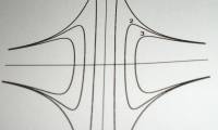
- Here is the finished chart image, with frame:

Part 3 of 3:
Helpful Guidance
- Make use of helper articles when proceeding through this tutorial:
- See the article How to Create a Spirallic Spin Particle Path or Necklace Form or Spherical Border for a list of articles related to Excel, Geometric and/or Trigonometric Art, Charting/Diagramming and Algebraic Formulation.
- For more art charts and graphs, you might also want to click on Category:Microsoft Excel Imagery, Category:Mathematics, Category:Spreadsheets or Category:Graphics to view many Excel worksheets and charts where Trigonometry, Geometry and Calculus have been turned into Art, or simply click on the category as appears in the upper right white portion of this page, or at the bottom left of the page.
Was this article helpful?
Your feedback helps us improve.
Related Articles
 How to Create a Curve in Excel13 minutes read
 How to Acquire a Lemniscate Curve of Sinewave Spheres in Excel17 minutes read
 This little trick can make your Widget invisible on iOS 142 minutes read
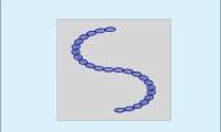 How to Create an S Curve Pattern in Microsoft Excel6 minutes read
 How to Make a Transparent Background in Canva for Free4 minutes read
Reader Comments 0
Sign in with email or Google to join the discussion.