How to Create a Floral Glassware Pattern in Microsoft Excel
In this article, you'll learn to make the 'floral glassware' pattern and image below, and the dozens of variations the file permits therefrom. Become familiar with the image(s) to be created: === Previous Lessons Learned ===
Part 1 of 4:
Previous Lessons Learned
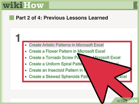
- This article relies on the previous accomplishment of the 6 articles preceding it:
- Create Artistic Patterns in Microsoft Excel
- Create a Flower Pattern in Microsoft Excel
- Create a Tornado Screw Pattern in Microsoft Excel
- Create a Uniform Spiral Pattern in Microsoft Excel
- Create an Insectoid Pattern in Microsoft Excel
- Create a Skewed Spheroids Pattern in Microsoft Excel
-
 Please complete those first before attempting this one.
Part 2 of 4:
The Tutorial
-
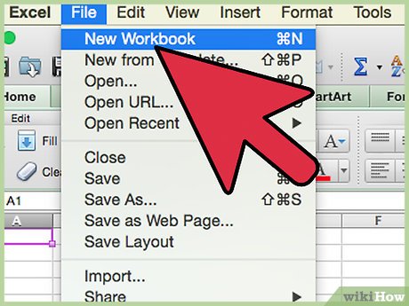
 Start a new workbook by saving the previous workbook under a new name. Save the workbook into a logical file folder.
 -
 Complete all changes in the upper Defined Variables section.
- Enter On=0,Off=1 cell A4 = 1
- Enter Adjuster = 1
- Enter TURNS = 9
- Enter S's Count = 4
- Enter Var = "=IF(S_COUNT<4,S_COUNT+30,12)"
- Enter Divisor = 3.0
- Enter top = "=ROUND((-B4*PI())+(Adj),0)" 968061
- Enter YN = Y
- Enter Power = 15. Insert New Comment "Try 1500^.5".
- All the rest are the same as they were before.
-
 Complete all changes in the upper Columnar Formulas section.
- c = -152,555 as the result of "=ROUND(-EXP((PI()^2)+(Cc*-(db))),0)+Designer"
- Enter to D7:D1447 w/ D7 active "=X7/Divisor+IF(COS((ROW()-7)*PI()/180*Factor)<0,ABS(COS((ROW()-7)*PI()/180*Factor))^Power*-1,COS((ROW()-7)*PI()/180*Factor)^Power)"
- Enter to E7:E1447 w/ E7 active "=Y7/Divisor+IF(SIN((ROW()-7)*PI()/180*Factor)<0,ABS(SIN((ROW()-7)*PI()/180*Factor))^Power*-1,SIN((ROW()-7)*PI()/180*Factor)^Power)"
- The External Ring and GMLL x,y and GMSL x,y formulas are unchanged. All other formulas and lookup tables are unchanged.
- Enter 1's Sequence to cell AB6 and Format Font Underline.
Part 3 of 4:
Explanatory Charts, Diagrams, Photos
-
 Create the Chart (dependent upon the tutorial data above).
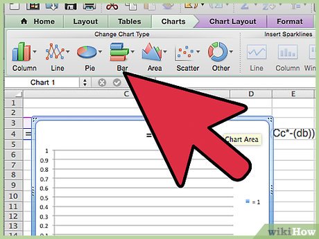
- Edit Go To cell range F7:G1446 on the Data worksheet and using Chart Wizard or the Ribbon, select Charts All/Other, Scatter, Smoothed Line Scatter. Copy the Chart to the Chart worksheet and expand it with the double-headed arrow via the bottom right corner.
- Select Chart Layout and get rid of the axes and grid lines and legend; select Data Series 1.
- Format Selection Line Weight 2, Solid Color Wheel Color Deep Purple, Transparency 0%.
- Select Plot Area and Format Selection Line - No Line, Fill-- Radial 4 colors: Left to Right: 1) Grey blend to 5/8 marker 2) Cerulean blue, then 3) tightly packed Navy blue, then last quarter = 4) Light Sky Blue.
- Glow - Dark Blue but not Navy Blue, Size 32 pt, Transparency 78%, Soft Edges 7 pt.
- 3-D Format - Surface: Translucent Powder, no Bevel.
- Select Chart Area and Format Selection:
- Fill Solid Navy Blue, Line - No Line, Shadow - Outer 315 degrees black Size 334 Blur 4 Pt Distance 30 pt Transparency 11%; Glow & Soft Edges - No, 3-D Format - None.
-
 But there's no reason to go with my hippie tastes! Format the chart as you please! Done!
 -
 Copy the live formulas and Paste Special Values then too to Saves, then Do Copy Picture and Paste Picture from the Chart with the Shift Key depressed to Saves and Save the workbook. Do so for each modification in the Tips section below.
 -
Part 4 of 4:
Helpful Guidance
- Make use of helper articles when proceeding through this tutorial:
- See the article How to Create a Spirallic Spin Particle Path or Necklace Form or Spherical Border for a list of articles related to Excel, Geometric and/or Trigonometric Art, Charting/Diagramming and Algebraic Formulation.
- For more art charts and graphs, you might also want to click on Category:Microsoft Excel Imagery, Category:Mathematics, Category:Spreadsheets or Category:Graphics to view many Excel worksheets and charts where Trigonometry, Geometry and Calculus have been turned into Art, or simply click on the category as appears in the upper right white portion of this page, or at the bottom left of the page.
Similar Post
- How to Create a Tornado Screw Pattern in Microsoft Excel
- How to Create the One Sphere Pattern in Microsoft Excel
- How to Create an Insectoid Pattern in Microsoft Excel
- How to Create a Necklace Pattern in Microsoft Excel
- How to Create a Different Necklace Pattern in Microsoft Excel
- How to Create an S Curve Pattern in Microsoft Excel


 Ways to install Microsoft Excel on Linux
  How to fix Office activation error 0xc004c060
  How to fix the Microsoft Teams shortcut not working on the computer
  Do not rush to update Patch Tuesday for November 2021 because it causes printer errors on Windows 10 again
  How to report Windows 11 errors, suggest Windows 11 features for Insider Preview users
  How to create exams on Microsoft Teams