How to Drawing Probability Distribution Charts in Excel

This updated guide explains how to Drawing Probability Distribution Charts in Excel through clear steps, practical examples, and important checks that help prevent common errors.

In order to use the Histogram Office, the Analysis Toolpak must be installed.

1. Install Analysis Toolpak

Step 1: click File -> Option -> Dialog appears -> at Add-Ins tab -> select Analysis Toolpak -> Go .

Step 2: The Add-Ins dialog box appears -> select the Analysis Toolpak -> OK .

So you have installed Analysis Toolpak for Excel.

2. Draw a Histogram of Probability Distribution Using Histogram

Example

Example: For a data table, draw a histogram of probability distribution using Histogram.

Step 1: Select Data -> Data Analysis -> The Data Analysis dialog box appears -> Histogram -> OK .

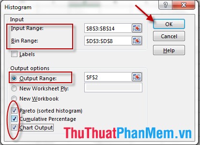
Step 2: Histogram dialog appears -> Select the data you may need to draw in Input Range -> Select the data area containing the value of the layers in Bin Range -> Select the position of the chart in Output Range -> Check all 3 items: Pareto , Cumulative , Chart Output -> OK .

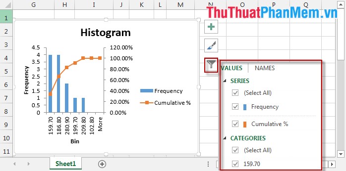
Results have drawn the chart:

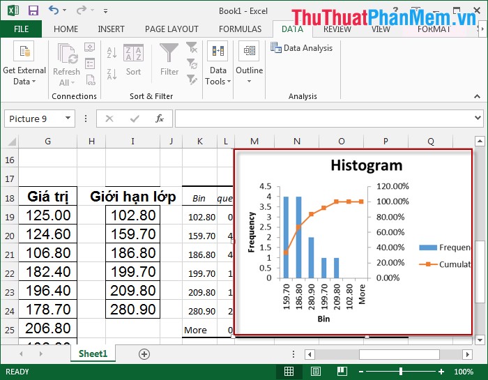
Working on the Chart

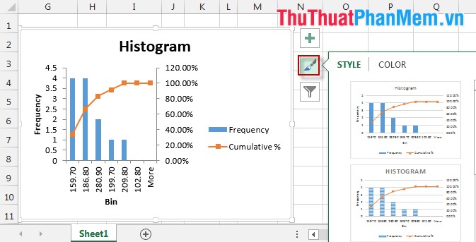
1. Change the Style and Color for the Chart

Click the icon

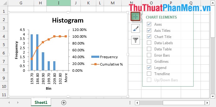
2. Add the Elements of the Chart

Example

For example: Add GridLines -> click the icon

3. Select the Values of the Chart

Click the icon