How to Learn Spreadsheet Basics with OpenOffice Calc

Method 1 of 3:

Open A Spreadsheet

If you are in a OpenOffice program, click File > New > Spreadsheet.
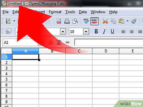
1. In either case a spreadsheet called Untitled1 appears on our screen.

Method 2 of 3:

The Calc Toolbars

The following four Calc Toolbars appear at the top of all Calc screens.

Examine the Main Menu Toolbar.
1. The first toolbar is the Main Menu toolbar that gives you access to many of the basic commands used in Calc.
Look at the Function Toolbar.
1. The second toolbar down is the Function Toolbar. The Function Toolbar contains icons (pictures) to provide quick access to commands like New, Open, Print, Copy, Paste, etc. When you place your mouse cursor over any of the elements of a toolbar, the name of the element appears on your screen.
2. Move your cursor over the icon . (The word 'New' appears. Clicking on opens a new spreadsheet.)
Check out the Formatting Toolbar.
1. The third toolbar down is the Formatting Toolbar. The Formatting Toolbar has icons plus drop-down menus that allow you to select a font, font color, alignments, number formats, border options and background colors.
See what the Formula Toolbar can do.
1. The fourth toolbar down is the Formula Toolbar. The Formula Toolbar contains the Name Box drop-down menu and a long white box called the Input Line.
2. Note: If your Toolbars look different, it is because these toolbars are in 800x600 screen resolution and the last eight icons are not shown but are available by clicking on the on the far right of the toolbar.

Method 3 of 3:

The Spreadsheet Itself

The rest of the window contains the spreadsheet. The spreadsheet is divided into rows that have a number at the left of each row and divided into columns with letters at the top of each column.

Learn the definition of a cell in spreadsheets.
1. A cell is the fundamental element of a worksheet. This is where things are added and where things are seen. A cell address in a spreadsheet identifies the location of the cell in the spreadsheet. A cell address is a combination of the column letter and the row number of a cell, such as A2 or B16.etc. When identifying a cell by its address, the column letter is always listed first followed by the row number. The cell address of the example below is A5.
Enter Data.
1. Click on the A1 cell (The cell at the very top left of the spreadsheet).
2. Notice the heavy black border around the A1 cell. The heavy black border indicates that A1 is the active cell. (A is at the top of the first column and 1 is on the first row. Both are highlighted. The highlighting also indicates that A1 is the active cell.)
3. Type Hello World and press Enter.
  1. The active cell is now A2. (The words 'Hello World' are in A1.)
4. When you type something in a cell and press Enter, what you typed is seen in that cell and the cell below becomes the next active cell.
Delete Data.
1. Click on A1 again.
2. Press the Delete key or right click the cell and select delete contents. (The 'Delete Contents' window appears.)
3. Check the Delete all box then click OK. ('Hello World' is deleted from A1)
Format Data
1. Separate Thousands, Two Decimal Places, Red Negative Numbers. Click cell A1. > Type the number -9999.129 > Press Enter. (The cursor moves to cell A2)
2. Right-click cell A1. (A small menu appears) > click Format cells. (The 'Format cells' window appears)
3. Click Numbers tab. Under 'Category', click on Number. Under 'Format', click on -1,234.12. Click In the small box before 'Negative numbers red'. (A check-mark appears in the box) > Click OK. (The number '-9,999.13' appears in cell A1.
4. Align Left, Click Alignment tab. In the 'Horizontal' pull-down menu, select Left. Click OK. (the numbers move to the left edge of the cell.)

Micah Soto

Update 05 March 2020

You should read it

May be interested

How to Create an OpenOffice Macro
an openoffice macro can be created to combine a series of frequently repeated tasks into a single step. macros can be effective in saving time, increasing efficiency, and improving productivity in situations where there is a significant...
How to Use Charts and Diagrams in OpenOffice Draw
draw offers no special toolbar for creating organization charts, where individual fields appear as rectangles. however, drawing these charts presents no special problems, however. the use of different fill colors clearly represents...
How to Draw Basic Shapes Using Open Office Draw
openoffice has its own suite of software that matches the versatility and strength of ms office and, being open source, it is free. read this article to learn how to draw basic shapes using openoffice draw. you can draw both 2d and 3d...
How to Use OpenOffice Writer
writer is the word processing feature in openoffice. this tutorial explains how to use the 'tips' feature, open a new text document, change paper size, change margins, change the indentation of paragraphs, use icons, close and open files,...
How to color formula cells in Excel automatically
coloring formula cells in excel helps us quickly identify cells that use formulas in long data tables.
Study online on e-Learning lectures
the e-learning lecture store under the ministry of education and training provides courses with various levels and subjects for students or teachers to have more teaching and learning materials.