Guide to splitting column data in Excel - into 2 or more columns in a table

Separating Excel data within columns, such as separating the full name column, is essential when creating student lists or other types of lists. Having information in the same column can make it difficult to read, resulting in unclear information and making it hard for users to understand.

Splitting data in Excel is relatively simple and almost the same as in other versions. However, in Excel 2013 and later, we have the Flash Fill tool to split data in Excel cells more easily and quickly. Below is a guide on how to split data in Excel across different versions.

1. Instructions for separating data in Excel 2013, 2016, and 2019

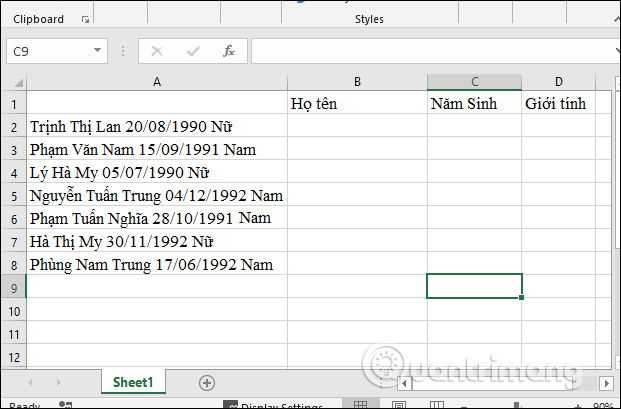
We will have the data table below with student information in a single column, and we need to separate it into three distinct columns: Full Name, Year of Birth, and Gender.

Method 1: Use the shortcut Ctrl + E for Flash Fill

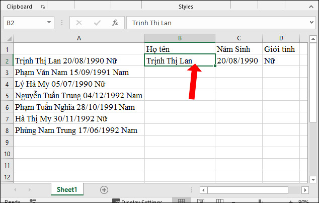
Step 1:

First, please enter the complete information for the first row in the data table.

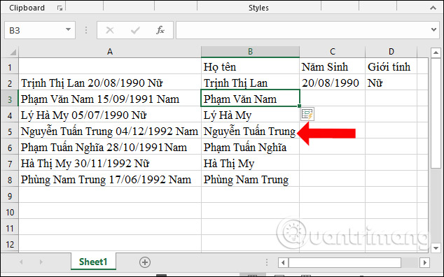
Step 2:

Next, press Enter to move to the next cell, then press Ctrl + E to complete the list of remaining names in each cell.

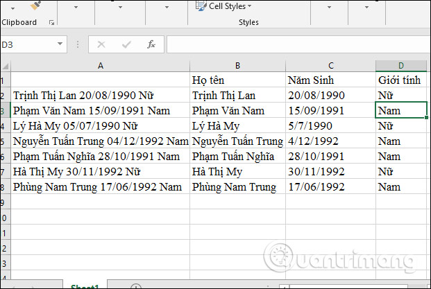
Do the same for the remaining two columns: Year of Birth and Gender.

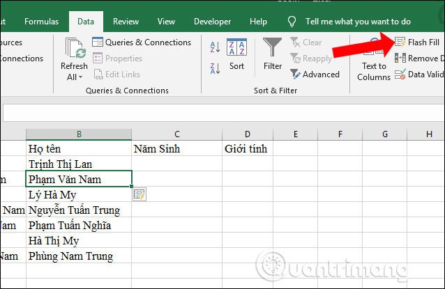
Method 2: Separate data using the Data Flash Fill menu.

Users also enter information in the first cell of the Full Name column, then click down to the second row. Next, click the Data tab on the ribbon and then click Flash Fill to enter the corresponding values ​​into the remaining cells in the column.

Method 3: Using the manual fill tool

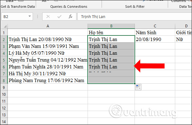
Step 1:

In the Username column, enter the information for the first cell. Then, hover your mouse over the first cell to display a plus sign in the bottom right corner of the cell and drag it down to the bottom of the column.

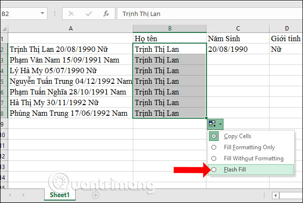
Step 2:

Then , a downward-pointing triangle icon will appear at the bottom corner of the column . Click on it and select Flash Fill from the displayed list.

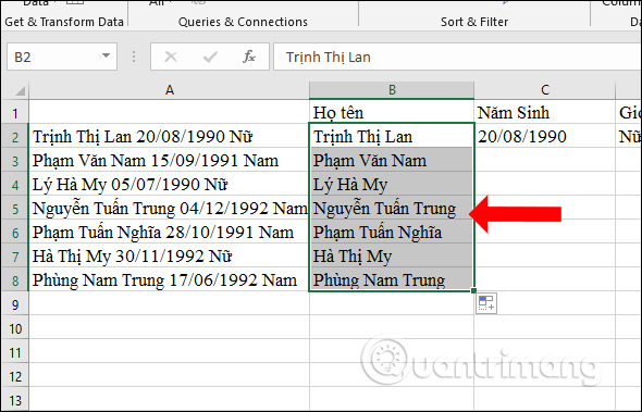
The correct values ​​will be immediately replaced as shown below. We perform the same operation with the Year of Birth and Gender columns.

The Flash Fill tool is only available in Word 2013 and later. The final manual method will provide more efficient and accurate values ​​for each cell compared to the two methods above. If you are using Office 2010 or earlier, use the Text to Columns tool as instructed below.

2. How to extract internal data in Excel cells in 2010 and 2007

In the table below, we have a column for full name followed by the score for each person. The full name is connected by a hyphen to the score in the same column. I will separate this information column into two distinct columns: one for full name and the other for score.

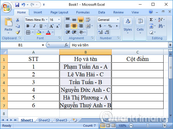
Step 1:

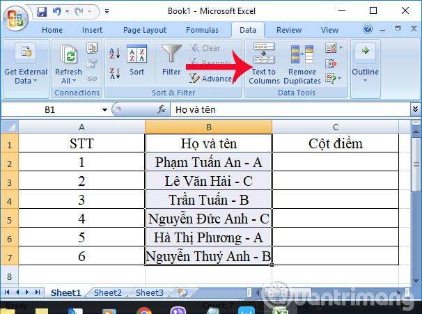
In your Excel spreadsheet, you need to highlight the area you want to separate into a different column. The header and unrelated content do not need to be highlighted. Then, click on the Data tab on the Ribbon, and then select Text to Columns .

Step 2:

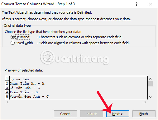
The Convert Text to Columns Wizard dialog box will appear. Here you will need to perform 3 steps to get the column you want to split. First, under Original data type , there will be 2 options for splitting columns:

1. Delimited: This method splits columns using delimiter characters such as tabs, hyphens, commas, spaces, etc.
2. Fixed with: splits columns according to the width of the data. For example, if the data consists of two columns, even though each row has a different length, the width is divided equally into two equal sections.

Since this article uses hyphens to separate content, I will check the "Delimited" option , then click " Next" below.

Step 3:

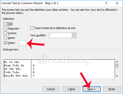
Next, go to the Delimiters section and select the content separator you want to use to separate the columns. The options include:

1. Tab: content is separated by a tab space.
2. Semicolon: spaced by semicolons.
3. Comma: Use commas as separators.
4. Space: Use a space to separate them.
5. Other: Use a different separator to separate the content.

Since the content uses hyphens to separate words, click on the "Other" option and then enter the hyphens used in the Excel file into the adjacent box. Then click " Next" to proceed to the final step.

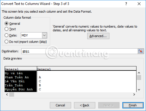
Step 4:

Immediately afterwards, you will see the results below in the Data preview section. If the requirements for splitting the content in the Excel column are met as you intended, Excel will proceed to split it into two separate columns. Then, you need to click on each cell to select the data format . For example, for the first cell, choose Text or General.

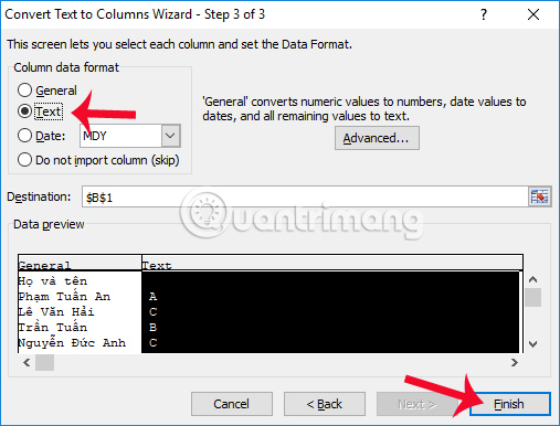
Change the format for the second cell to Text as well. Finally, click Finish at the bottom to complete the setup for separating the content in Excel.

Step 5:

Then a notification window will appear as shown below; we press OK to agree.

Thus, the content in one column of the Excel table has been split into two columns with different content, as shown in the image below.

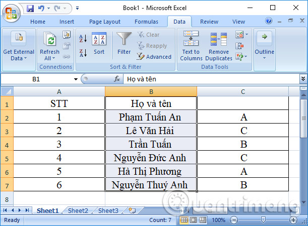
Thus, we have completed the process of splitting the content in a column in Excel into two separate columns. Splitting content in a column in Excel is a basic operation that is frequently performed. This will make the content in the table easier to follow and observe.

Good luck with your project!

You've just finished reading the article "Guide to splitting column data in Excel - into 2 or more columns in a table" edited by the TipsMake team. You can save guide-to-splitting-column-data-in-excel-into-2-or-more-columns-in-a-table.pdf to your computer here to read later or print it out. We hope this article has provided you with many useful tech tips and tricks. You can search for similar articles on tips and guides. Thank you for reading and for following us regularly.