How to use the WRAPCOLS function in Excel

Want to split a long list into multiple columns? So let's learn how to use the WRAPCOLS function in Microsoft Excel .

How to use the WRAPCOLS function in Excel Picture 1

There are many functions in Microsoft Excel that can help sort numbers and data. One of these functions is WRAPCOLS. This function gives Excel users an exciting new way to quickly convert their column into a 2D array, thereby improving readability and data visualization.

What is the WRAPCOLS function in Excel?

The WRAPCOLS function works by combining row and column values ​​into a two-dimensional column array. You will specify the length of each column in the formula.

This is a new dynamic array function in Excel. It is available to all Microsoft 365 subscribers, including the basic plan.

Syntax of WRAPCOLS function in Excel

The syntax of the WRAPCOLS function has the following arguments:

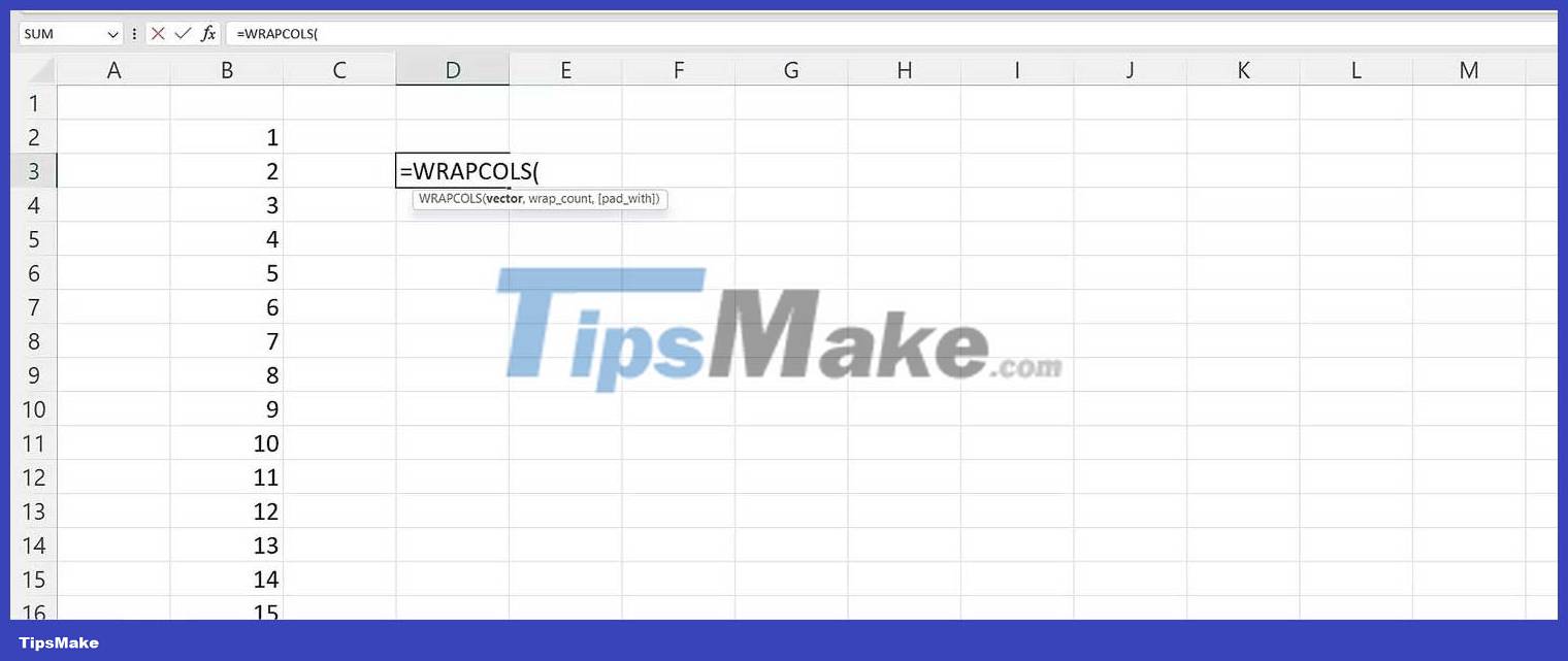
=WRAPCOLS(vector, wrap_count, [pad_with])

Specifically:

1. Vector represents the reference or range of cells you want to include.
2. wrap_count is the maximum number of values ​​for each column.
3. pad_with is the value you want to add to the row. In Excel, the default is #N/A if no data is specified.

How to use the WRAPCOLS function in Excel

To get started, you need sample data. You can use one of several ways to number rows in Excel when you want to get a list of numbers from 1 to 20. To include these numbers into a 2D array, you can use the WRAPCOLS function.

1. Write the formula in a cell or through the formula bar =WRAPCOLS( .

How to use the WRAPCOLS function in Excel Picture 2

2. Select the array of numbers and write a comma.

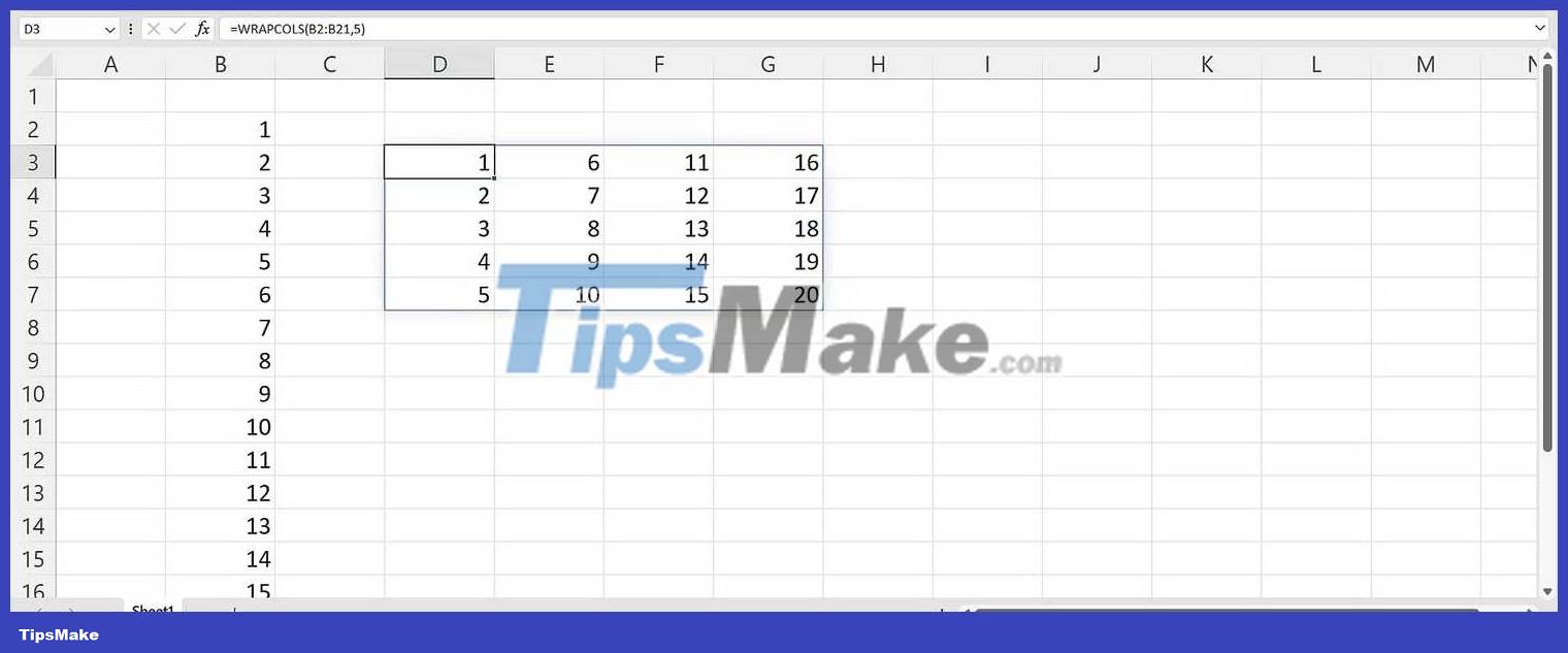
3. For the wrap_count argument , write 5. This will split the number into columns, where each column contains 5 values.

4. Close brackets.

5. Press Enter on the keyboard.

The final syntax is:

=WRAPCOLS(B2:B21,5)

How to use the WRAPCOLS function in Excel Picture 3

How to use pad_with argument in WRAPCOLS . function

By default, Excel throws a #N/A error if the number of values ​​has expired and is not equal to the number you specified in wrap_count.

What does that mean? Replace 4 with 7 in the original formula. The syntax will be as follows:

=WRAPCOLS(B2:B21,7)

How to use the WRAPCOLS function in Excel Picture 4

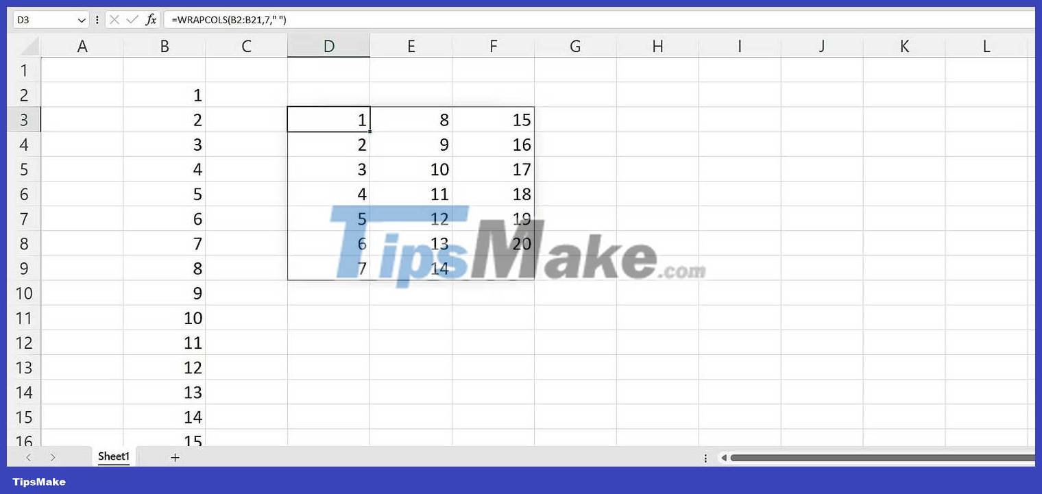
The #N/A error that appears means all values ​​from the source have been taken into account. To make sure that error doesn't appear again, specify a value for the pad_with argument. To make this work:

1. Write WRAPROWS( .
2. Select the range of numbers, and then add a comma.
3. Write 7 for the wrap_count argument .
4. Add commas.
5. For the pad_with argument , write a " " sign , representing the distance.
6. Press Enter on the keyboard.

The final syntax would be:

=WRAPCOLS(B2:B21,7," ")

How to use the WRAPCOLS function in Excel Picture 5

Example case using WRAPCOLS . function

Now let's consider a situation where suppose you have a list of dates that you want to split into 4 parts. You can use the WRAPCOLS function. Proceed as follows:

1. Write this function.
2. Select range. They will be dates.
3. Choose 3 as the wrap_count argument .
4. You can add spaces, even dashes as the pad_with argument .
5. Finally, press Enter on the keyboard.

The final syntax would be:

=WRAPCOLS(C2:N2,3)

Even if your data is inconsistent in Excel, you can still include and organize them into columns. Just select the desired number of values ​​in each column, and then press Enter.

In addition to the Excel WRAPCOLS Function, you can also use WRAPROWS to break data into rows.

Hope the article is useful to you!

Isabella Humphrey

Update 24 July 2023