How to use the IMPORTRANGE function in Google Sheets

If you work with Google Sheets often enough, you'll inevitably need to transfer data from one spreadsheet to another.

The IMPORTRANGE function in Google Sheets helps us link data from different spreadsheets, allowing for quick data searches and retrieving data according to the function's specifications. Therefore, you can use the IMPORTRANGE function to quickly extract and link data across Google Sheets spreadsheets.

Using the IMPORTRANGE function in Google Sheets is simple and can be combined with other functions . This article will guide you on how to use the IMPORTRANGE function in Google Sheets.

The structure of the IMPORTRANGE function in Google Sheets

Google Sheets IMPORTRANGE function structure

=IMPORTRANGE('spreadsheet_url'; 'cell_range_string')

In there:

1. Spreadsheet key: a long string of numbers and letters in the URL for a specific spreadsheet.
2. Spreadsheet URL: This is the address link to a specific spreadsheet file.
3. Range string: is the exact name of the spreadsheet from which to retrieve data, followed by '!' and the range of cells from which to retrieve data.

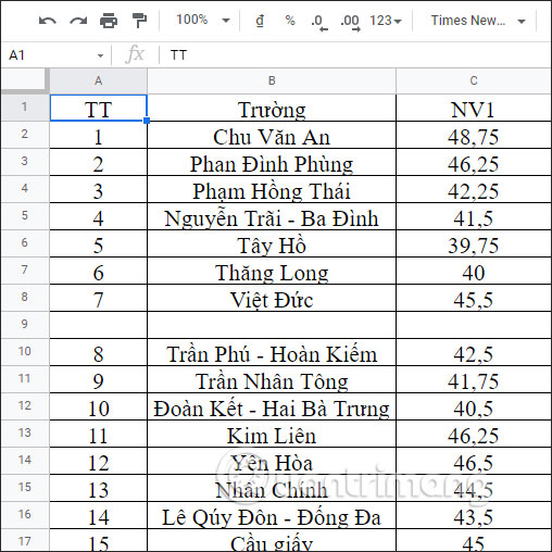
Let's take the example of the Grade 10 Benchmarks 2019 data table, with the requirement to extract data from cells B2 to C29 in the spreadsheet on Page 1.

You need to open a completely new spreadsheet in Google Sheets to retrieve the data you need. First, you need to copy the link to the document "Grade 10 Entrance Exam Scores - 2019" .

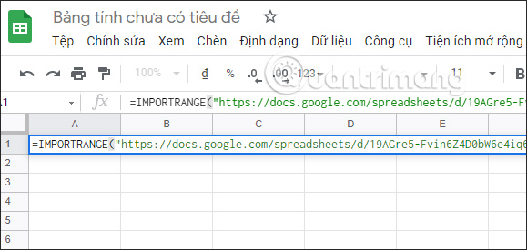
Next, in the new spreadsheet interface, enter the function formula as shown below and press Enter.

=IMPORTRANGE("https://docs.google.com/spreadsheets/d/19AGre5-Fvin6Z4D0bW6e4iq6yYX13kar0EIvXAVh-VQ/edit#gid=887314864"; "Page1!B2:C29")

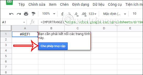
You will immediately see the #REF! message . You need to click on this message and click Allow access to grant the IMPORTRANGE function permission to access data from another worksheet.

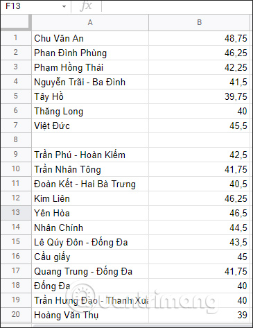
The data from the worksheet you selected is now displayed on another worksheet, as shown below.

How to use the IMPORTRANGE function in Google Sheets

1. With just two arguments, using the IMPORTRANGE function is usually quite straightforward. Let's say you have a spreadsheet and you want to import it into a new spreadsheet.

2. Click on the URL in the address bar at the top of your browser and copy it. Alternatively, you can simply copy the spreadsheet key from within the URL.

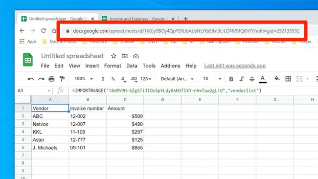
3. In the new spreadsheet, enter "=IMPORTRANGE(" - without quotation marks.

4. Paste the URL and add double quotes (").

5. Enter a comma, add double quotes ("), and enter the range of cells you want to include. It will look like this: "Sheet1!B1:C6". Here, it specifies that, for example, you want the spreadsheet named "Sheet1" and want the cells from B1 to C6.

6. Add a closing parenthesis and press Enter.

7. The complete function will look like this:

=IMPORTRANGE("https://docs.google.com/spreadsheets/d/1Zoq0M0RG-RLYZ9HjOf01ff9eSPIYY3s/edit#gid=1027643093", "Sheet2!A1:C12")

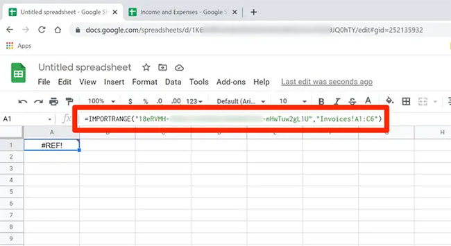
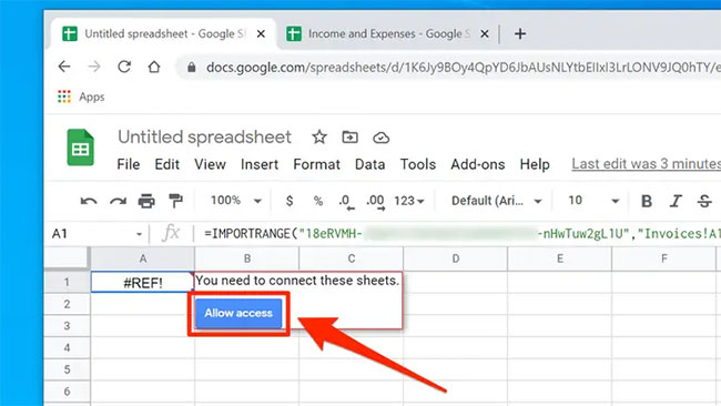
8. However, you may notice that the data isn't being imported – there's a #REF! error in the replacement cell. Click on this cell and you'll see a message that you need to connect the worksheets. Click "Allow access" and then the data will appear. You'll only need to do this once for each worksheet from which you import data.

How to use the IMPORTRANGE function with the QUERY function.

By combining the IMPORTRANGE function with the QUERY function, you can retrieve data precisely based on the criteria you need to extract.

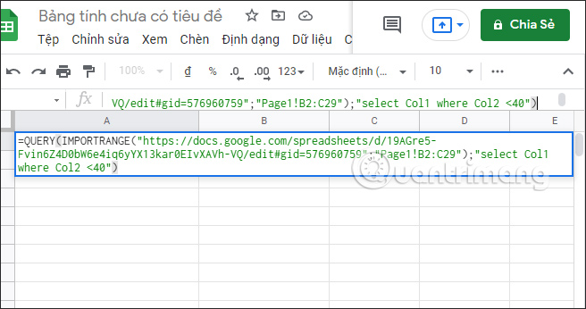
We will select the data from cell B2 to cell C29 in the spreadsheet on Page 1 and only take column NV1. Enter the formula as below and press Enter.

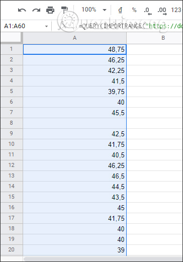
=QUERY(IMPORTRANGE("https://docs.google.com/spreadsheets/d/19AGre5-Fvin6Z4D0bW6e4iq6yYX13kar0EIvXAVh-VQ/edit#gid=576960759";"Page1!B2:C29");"SELECT Col2") 

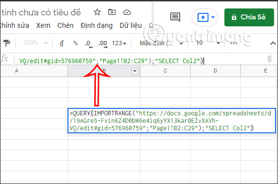
The results will only display the NV1 score column.

Alternatively, you can also use the scores of schools with first-choice admission scores.

We enter the function formula as shown below and then press Enter.

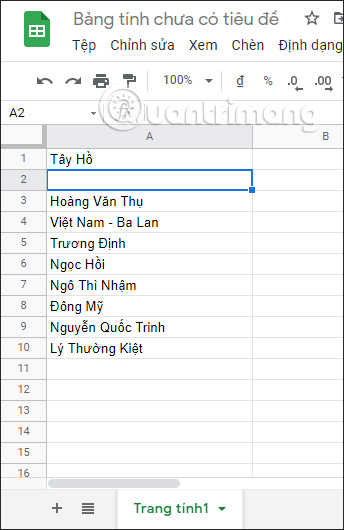
=QUERY(IMPORTRANGE("https://docs.google.com/spreadsheets/d/19AGre5-Fvin6Z4D0bW6e4iq6yYX13kar0EIvXAVh-VQ/edit#gid=576960759";"Page1!B2:C29");"Sect Col1 where Col2 <40") 

The results will display the names of schools whose first-choice admission scores are lower than 40 points.

An example of how to use the IMPORTRANGE function in Google Sheets.

Use IMPORTRANGE with URL or Spreadsheet Keys

Suppose you have multiple different Google Sheets spreadsheets containing test scores for students in different subjects (for example, one spreadsheet for Math scores and another for English scores, etc.).

If you want to combine all these sheets and have the data in the same sheet, you can use the IMPORTRANGE function.

Step 1 : Before using the formula, you need to get the URL of the Google Sheets document where you want to import the data. You can find that URL in the browser's address bar when the Google Sheets document is open.

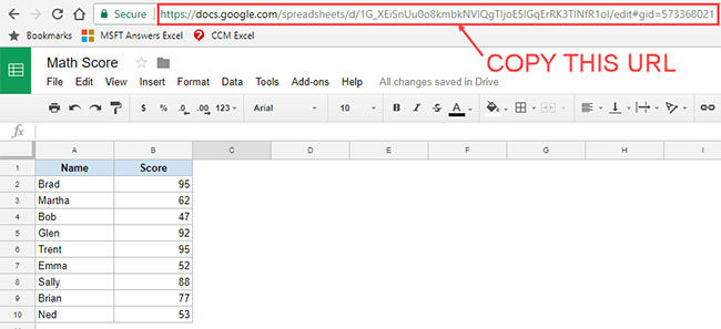
Alternatively, you can also copy the short key from the URL instead of the full URL (as shown below). This guide will use the short key in the formula.

Step 2 : Enter the function and paste the URL or short key to add the first argument to the syntax.

Step 3 : Enter commas and specify the range for entering them.

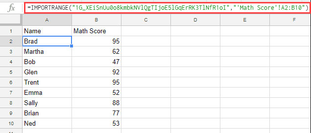
Below is the Google Sheets IMPORTRANGE formula that will allow you to enter students' names and scores into the current worksheet using the short key from the URL above:

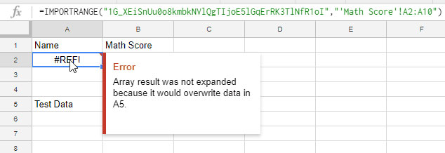
=IMPORTRANGE("1G_XEiSnUu0o8kmbkNVlQgTIjoE5lGqErRK3TlNfR1oI","'Math Score'!A2:B10")

Note that the second argument of this formula is "'Math Score'!A2:B10". In this argument, you need to specify the worksheet name as well as the range (enclosed in quotation marks).

Step 4 : When you first enter this formula, you will see a #REF! error in the spreadsheet. When you hover your mouse over the cell, you will see a prompt asking you to allow access ("Allow access").

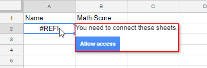
Click the blue button and it will give you the results. Note that this only happens once per URL. Once you have granted access, the request will not repeat.

This can be useful if you need to retrieve data from multiple spreadsheets. For example, in this case, you could retrieve grades for all subjects from different Google Sheets into a single spreadsheet.

Use the IMPORTRANGE function with Named Range

If you have to import ranges from multiple sources, it's easy to get confused. However, you can name the ranges to make things a little easier. Just follow this procedure:

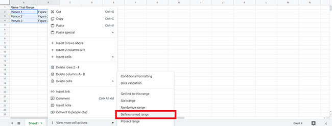
Step 1 : In the worksheet where you want to import the text, highlight the range of cells and right-click on it, then navigate to More cell actions > Define named range .

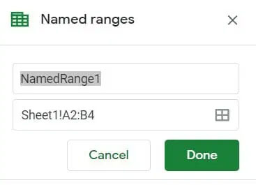
Step 2 : In the pop-up menu, name the range.

Step 3 : In the new worksheet, use the Google Sheets IMPORTRANGE function with the range named range_string. In the example, the command would be as follows:

=IMPORTRANGE("1G_XEiSnUu0o8kmbkNVlQgTIjoE5lGqErRK3TlNfR1oI","'NamedRange1")

Step 4 : Press Enter , then click on the #REF error and click Allow Access.

Some notes and tips on using the IMPORTRANGE function in Google Sheets.

Once the worksheets are connected (because you've granted access the first time you used the formula), any updates made in any worksheet will automatically be reflected as the formula's result. For example, if you edit a student's grade, it will automatically change in the sheet containing the formula.

When using the IMPORT RANGE formula, ensure there are enough empty cells to hold the result. If you have some data in a cell that matches a cell needed for the formula's result, the formula will return an error. However, it helps identify the error by letting you know the problem when you hover your mouse over the cell.

If you're importing data from multiple spreadsheets, this can be a bit confusing. It's a good practice to create Named Ranges in the source sheet and then use the named ranges.

If you want that data to be added to the source page, instead of dragging a specific range, drag the entire column. This will retrieve data from both columns A and B. Now, if you add more data to the source page, it will automatically update in the destination page.

Frequently Asked Questions about the IMPORTRANGE function in Google Sheets

How do I use the IMPORTRANGE function in Google Sheets?

1. Find the URL in your browser's address bar to enter.

2. Enter =IMPORTRANGE( into an empty box and paste the URL inside the quotation marks.

3. Enter a comma, then specify the range inside the quotation marks, for example: 'Sheet2!B6:C18' and press Enter.

4. Click on the #REF error and then click on Allow Access .

What is the IMPORTRANGE function in Google Sheets?

IMPORTRANGE is a function that allows you to transfer data from one spreadsheet to another without having to manually enter it. Using this function is better than copy-pasting because it updates automatically.

Does the IMPORTRANGE function automatically update Google Sheets?

Yes, any changes made to the original spreadsheet will also change the data that has been imported.

Are there any limits to the IMPORTRANGE function in Google Sheets?

Yes, there can be up to 50 cross-referenced recipes in the workbook.

How do I filter the IMPORTRANGE function in Google Sheets?

You should use the QUERY function to filter information from the entered data.

How do I use multiple IMPORTRANGE functions in Google Sheets?

Follow the standard procedure for importing a range of cells, but ensure that each time you use the IMPORTRANGE function, there is enough space in the worksheet to display the data.

Can you use the formatted IMPORTRANGE function?

No, you can only enter that data itself.