SUMIF Not Working in Excel? Common Errors and Fixes

SUMIF adds values whose corresponding cells meet one condition. When it returns zero, the wrong total, or an error, the cause is usually the formula structure, the stored data type, a mismatched range, or the way the criterion was written.

Check the syntax and range sizes

=SUMIF(range, criteria, [sum_range])

• range contains the values to test.
• criteria defines the match.
• sum_range contains the values to add. If omitted, Excel adds matching numeric cells in range.

Keep range and sum_range the same size and aligned to the same rows. For multiple conditions, use SUMIFS, whose argument order differs: =SUMIFS(sum_range,criteria_range1,criteria1,...).

Write date criteria as real dates

Assume A2:A20 contains real Excel dates and C2:C20 contains quantities.

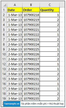
Prefer a date cell, such as F3:

=SUMIF(A2:A20,F3,C2:C20)

Or build an unambiguous date:

=SUMIF(A2:A20,DATE(2013,3,1),C2:C20)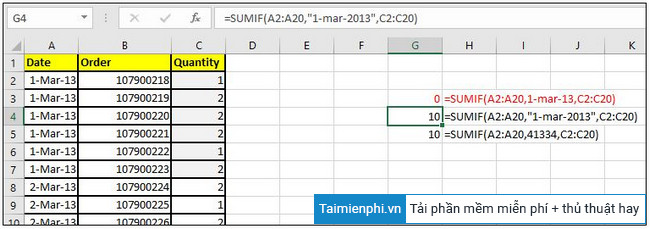

Do not hard-code a locale-dependent text date unless you know how that workbook interprets it. Formatting a text string to look like a date does not convert it into a date serial number.

Join comparison operators to values correctly

Put an operator inside quotation marks. When the comparison value is in F3, join it with &:

=SUMIF(A2:A20,">"&F3,C2:C20)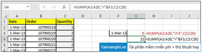

For a fixed number, =SUMIF(B2:B20,">100",C2:C20) is valid. For text, use quotation marks: =SUMIF(B2:B20,"East",C2:C20).

Convert numbers stored as text

SUMIF ignores text in the sum range, even when it looks numeric.

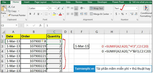
If Excel displays an error indicator, select the affected cells and choose Convert to Number.

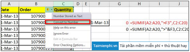
For imported data, use VALUE, Text to Columns, or a controlled multiply-by-1 conversion, then paste values if appropriate.

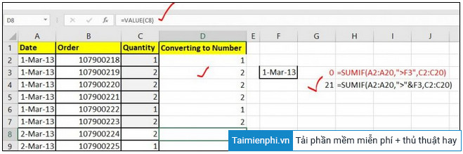
Also remove hidden spaces from criteria data with TRIM or CLEAN when exact text matches fail.

Format summed durations correctly

Excel stores time as fractions of a day. A valid formula can appear wrong if the result cell uses an unsuitable format.

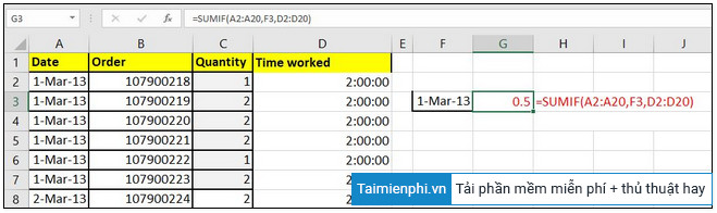
For totals that may exceed 24 hours, format the result as [h]:mm:ss rather than hh:mm:ss.

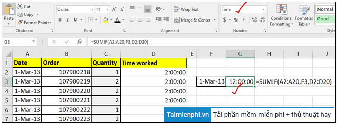
If the input times are text, convert them to numeric time values before summing.

Use SUMPRODUCT only for a clear reason

For aligned numeric ranges, this formula can perform an equivalent date match:

=SUMPRODUCT((A2:A20=F3)*D2:D20)

SUMPRODUCT is useful for array-style logic, but it does not repair dirty data automatically. Keep all arrays the same size and avoid full-column arrays in large workbooks.

Check external workbook references

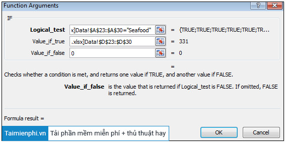
SUMIF and SUMIFS can return #VALUE! when they reference ranges in a closed source workbook. Open the source workbook, verify and save the links, or redesign the report with a supported import method such as Power Query. Do not replace the formula with an unrelated nested IF/SUM expression without testing the result.

Handle criteria longer than 255 characters

SUMIF/SUMIFS can return incorrect results for criteria strings longer than 255 characters. Shorten the match where possible, reference a helper key, or split a literal with &:

=SUMIF(B2:B12,"first part"&"second part",C2:C12)

Quick diagnostic checklist

1. Evaluate the criterion cell with =ISNUMBER(cell) or =ISTEXT(cell).
2. Confirm range and sum_range have identical dimensions.
3. Test the criterion with COUNTIF before adding values.
4. Use Formulas > Evaluate Formula to inspect each step.
5. Recalculate with Ctrl + Alt + F9 if calculation mode is manual.

For the basic formula pattern, see the SUMIF guide. For counting rather than summing, use the COUNTIF conditional counting guide.