How to Create Nearly Concentric Rings of Sinewave Spheres
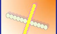
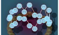
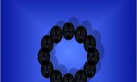
You'll learn how to create nearly concentric rings if sinewave spheres and create images like the one below, plus many more, by following these steps. Become familiar with the basic image to be created: === The Tutorial ===
Table of Contents
Part 1 of 3:
The Tutorial
-
 If you have completed the article and workbook, How To Create a Chaos Ring of Sinewave Spheres, you may SAVE AS that workbook under a new appropriate name for this project and look for NEW or MODIFIED notes in the article text, which follows the previous article prior to deviating from it. Otherwise simple follow the steps as given and open a new workbook and create three worksheets: Data, Chart (unless working with Chart Wizard), and Saves.
 - Set Your Preferences: Open Preferences in the Excel menu and follow the directions below for each tab/icon.
- In General, set R1C1 to Off and select Show the 10 Most Recent Documents .
- In Edit, set all the first options to checked except Automatically Convert Date System . Set Display number of decimal places to blank (as integers are preferred). Preserve the display of dates and set 30 for 21st century cutoff.
- In View, click on show Formula Bar and Status Bar and hover for comments of all Objects . Check Show gridlines and set all boxes below that to auto or checked.
- In Chart, allow show chart names and set data markers on hover and leave the rest unchecked for now.
- In Calculation, Make sure Manually and calculate before save are checked. Set max change to .000,000,000,000,01 without commas as goal-seeking is done a lot. Check save external link values and use 1904 system, Command + = performs a calculation session.
- In Error checking, check all the options.
- In Save, select Save preview picture with new files and Save Autorecover after 5 minutes
- In Ribbon, keep all of them checked except Hide group titles and Developer .
- Place the cursor at cell A16 and do Freeze Panes. Edit Go To cell range A1:N17288 and Format Cells Number Number Decimal Places 4, Font Size 9 or 10, Fill (from the color wheel) a nice fuchsia and make the Border Dark Blue bold Outline.
-
 Enter the upper Defined Name Variables Section (here's a picture):
- MODIFIEDL: Cell A1: Enter Sinewave Spheres in a Ring to 100
- B2: Enter Pasted and C2: Enter Values. Format Fill Red and Font White.
- E1: AYE
- E2: BEE
- E3: CEE
- F1: 10
- F2: .50
- F3: .50
- Select cell range E1:F3 and Insert Name Create Names in Left Column, OK.
- MODIFIED: G1: Stretch_x1 or cut and paste,
- MODIFIED: G2: Stretch_y1 or cut and paste
- MODIFIED: H1: Enter "=(8.5*(SHRINKER*10))" or cut and paste
- MODIFIED: H2: Enter "=(8.5*(SHRINKER*10))" or cut and paste
- G3: Shrinker
- H3: Enter "=0.1*12/SPHERES"
- MODIFIED: Select cell range G1:H3 and Insert Name Create Names in Left Column, OK.
- I1: ROWS
- I2: MAGIC
- I3: SPHERES
- J3: 56
- Select cell range I1:J3 and Insert Name Create Names in Left Column, OK.
- J1: Enter "=17285-5"
- NEW: J2: Enter "=ROUND(ROWS/SPHERES,0)"
- MODIFIED: Enter the column heading of rows 4 and 5:
- A5: Adj Cos (for Adjusted Cosine)
- B4: Enter 0 and Insert Name Define Name Adj_Sin to cell $B$4.
- B5: Adj Sin
- C5: Indicator
- NEW: D4: Enter .=RANDBETWEEN(4,7)/100 where if the period is deleted the formula becomes active.
- D5: Randy (for RandBetween)
- E5: t: 0 to nπ
- F5: z1_
- G5: Adj_x1
- H5: Adj_y1
- I4 and J4: Charting
- I5: x: No z
- J5: y: With z
- K5: Adj_x2
- L5: Adj_y2
- M4 and N4: Charting
- M5: x2: No Z
- N5: y2: With z.
- Command+Select cells F1:F3 and I3 and Format Fill yellow.
- Select cell J3 and Format Fill light sky blue from the color wheel.
- Select cell range I4:J5 and Format Font italic.
- Select cell range M4:N5 and Format Font italic.
- Command+Select cells A1:D1, A2, A3:D3, D2, G1:N2, G3:H3, M3:N3 and Format Fill White.
- NEW: Insert NEW COLUMNS and move Randy.
- Select columns K and Insert Column, Select Columns D;E and Insert Columns.
- Cut the Randy column, now column F, and paste it in the new column M.
-
 Enter the new Defined Variables in M1:L3 and O4; here's a picture:
- M1: Enter "=AYE" and Format Fill yellow for input.
- N1: Enter AYE2_
- M2: Enter "=ROUND(ROWS/SWS2_,0)"
- N2: Enter Magic2
- M3: Enter "=SPHERES*SWS_Factor" for now and Format Fill medium sky blue.
- N3: Enter SWS2_ (for SineWaveSpheres2)
- Select M1:N3 and Insert Names Create Names in Right Column, OK.
- O1: Enter "=(-1+SQRT(5))/2" and Insert Name Define Name GMLL for cell $O$1 for Golden Mean Long Leg.
- O2: Enter SWS Factor
- O3: Enter 1 for now, Been having problems getting this to work at .5,. 25, etc. The idea is to enter 56 or so Spheres and then .25*56 = 14 for the next inner circle.
- O4: Enter the formula w/o quotes, "=VLOOKUP(SWS2_*IF(SWS_Factor<>0,1/SWS_Factor,1),LOOKSTER2,2)*
IF(SWS_Factor<1,-2,1)*0"
-
- P1: Stretch_x2
- P2: Stretch_y2
- P3: Shrinker2
- Q1: Enter "=Stretch_y2)"
- Q2: Enter "=(8.5*(Shrinker2*10))"
- Q3: Enter "=(0.1*12/SWS2_)*VLOOKUP(SWS2_*IF(SWS_Factor<>0,
1/SWS_Factor,1),LOOKSTER2,3)*IF(SWS_Factor<1,GMLL,1)"
-


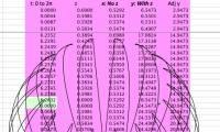
 Enter the new Lookup Table. Here's a picture (outlined areas are copied, yellow filled areas are series, open-ended outlined areas may be from series -- I forget. Not all have been tried, so if you find a discrepancy, please report back to us all-- thanks. They should be close though.) I suggest the table be entered in cell range T1:W103. Define Name LOOKSTER as the range T3:W103 and LOOKSTER2 as the range U3:W103 in that case.
 - NEW OR MODIFIED: Enter the column formulas - BE VERY CAREFUL TO COPY AND PASTE VALUES as specified please.
- Adj Cos: Edit Go To cell range A6:A17285 and enter into A6 w/o quotes the following formula, "=17*COS((ROW()-6)*0.25/12*PI()/180)" and Edit Fill Down.
- NEW: Adj Sin: Edit Go To cell range B6:B17285 and enter into B6 w/o quotes the following formula,"=17*SIN((ROW()-6)*0.25/12*PI()/180)+Adj_Sin"and Edit Fill Down.
- Indicator: Select cell C6 and enter 1. Edit Go To cell range C7:C17286 and enter w/o quotes the formula, "=IF((ROW()-7)/MAGIC=INT((ROW()-7)/MAGIC),1,IF((ROW()-7)=0,1,0))" and Edit Fill Down.
- Indicator2: Select cell D6 and enter 1. Edit Go To cell range D7:D17286 and enter w/o quotes the formula, "=IF((ROW()-7)/Magic2=INT((ROW()-7)/Magic2),1,IF((ROW()-7)=0,1,0))" and Edit Fill Down.
- t2: 0 to nπ: Select cell E6 and enter 0. Select cell E7 and enter the formula "=(2*PI()/Magic2)". Edit Go To cell range E8:E17285 and enter w/o quotes into E8 the formula "=IF(D8=1,2*PI(),2*PI()/Magic2+E7)" and Edit Fill Down.
- z2_: Edit Go To cell range H6:H17285 and copy it and paste it to F6. Enter w/o quotes into F6 the formula "=CEE*COS(AYE2_*E6)" and Edit Fill Down. Edit Go To cell range F6:F17285 and Insert Name Define Name z2_ to cell range $F$6:$F$17285.
- t: 0 to nπ: Select cell G6 and enter 0. Select cell G7 and enter the formula "=(2*PI()/MAGIC)". Edit Go To cell range G8:G17285 and enter w/o quotes into E8 the formula "=IF(C8=1,2*PI(),2*PI()/MAGIC+G7)" and Edit Fill Down.
- z1_: Edit Go To cell range H6:H17285 and enter w/o quotes into H6 the formula "=CEE*COS(AYE*G6)" and Edit Fill Down. Edit Go To cell range H6:H17285 and Insert Name Define Name z1_ to cell range $H$6:$H$17285.
- Adj_x1: Edit Go To cell range I6:J17285 and enter w/o quotes into I6 the formula "=IF(C6=1,A6,I5)" and Edit Fill Down. Edit Go To cell range I6:I17285 and Insert Name Define Name Adj_x1 to cell range $I$6:$I$17285.
- Adj_y1: Edit Go To cell range J6:H17285 and enter w/o quotes into J6 the formula "=IF(C6=1,B6,J5)" and Edit Fill Down. Edit Go To cell range J6:J17285 and Insert Name Define Name Adj_y1 to cell range $J$6:$J$17285.
- x: No z: Edit Go To cell range K6:K17285 and enter w/o quotes into K6 the formula "=SHRINKER^2*(Stretch_x1*(((BEE^2-CEE^2*COS(AYE*G6)*COS(AYE*G6))^0.5* COS(G6)))+Adj_x1" and Edit Fill Down.
- y: With z: Edit Go To cell range L6:L17285 and enter w/o quotes into L6 the formula "=SHRINKER^2*(Stretch_y1*(((BEE^2-CEE^2*COS(AYE*G6)*COS(AYE*G6))^0.5* SIN(G6))+z1_)+Adj_y1)" and Edit Fill Down.
- MODIFIED: Randy: Edit Go To cell range M6:M6918 and enter into M6 3 and into M6918 .5999 and do Edit Fill Series Column Linear Trend, OK. Edit Go To cell range M6918:M17285 and enter 4.5 into cell M17285 and Edit Fill Series Column Linear Trend OK. This is left over from the last image of the previous article but it occurred that you might like to have it.
- Adj_x2: Edit Go To cell range N6:N17285 and enter w/o quotes into N6 the formula "=IF(D6=1,A6,N5)" and Edit Fill Down.
- Adj_y2: Edit Go To cell range O6:O17285 and enter w/o quotes into O6 the formula "=IF(D6=1,B6+Aj,O5)" and Edit Fill Down.
- x2: No z: Edit Go To cell range P6:P17285 and enter w/o quotes into P6 the formula "=Shrinker2^2*(Stretch_x2*(((BEE^2-CEE^2*COS(AYE2_*E6)*COS(AYE2_*E6))^0.5* COS(E6)))+Adj_x2)" and Edit Fill Down.
- y2: with z: Edit Go To cell range Q6:Q17285 and enter w/o quotes into Q6 the formula "=Shrinker2^2*(Stretch_y2*(((BEE^2-CEE^2*COS(AYE2_*E6)*COS(AYE2_*E6))^0.5* SIN(E6))+z2_)+Adj_y2)" and Edit Fill Down.
- Select cell K17286 and enter the formula w/o quotes "=K6" and select cell L17286 and enter the formula w/o quotes "=L6". This makes the top connecting line from the last sphere to the first. Copy cell range K17286:L17286 and paste it to P17286.
- Edit Go To cell range K6:L17288 and do Format Fill sky blue. Edit Go To cell range P6:Q17288 and Format Fill sky blue.
- Select cell M5 and Format Fill light sea green, font red, Border navy blue outline bold. Copy this cell to J17287. Then do Edit Paste Special Format of this cell to cell C6, D6, E6, E7, G6, G7, K17286, L17286, P17286 and Q17286 to make distinct the format of those cell's formulas/values.
- Copy cell range A11:J17285 and then PASTE SPECIAL VALUES right back atop the same cell range. Format Fill Red and Font White. This means that the top Variables section is no longer operative in any useful way until you Edit Fill Down the formulas from row 10, which may mean having o wait a considerable length of time, as in 25 - 40 minutes. It can also take that long to save the workbook, so ...
- Save the workbook. Suggested filename is Sinewave Spheres in Rings.
Part 2 of 3:
Explanatory Charts, Diagrams, Photos
- (dependent upon the tutorial data above)
- Create the Chart.
- Enter to cell L3 60 if not already done.
- Select cell range K6:L17285, and either Insert Chart or select Charts from the Ribbon,
- Select chart type Scatter, Smooth Line Scatter, and a chart will appear atop your worksheet.
- Select cell range P6:Q17285 and do command and c, Copy.
- Click on the existing circle of spheres in the existing chart you just made and do command and v, paste. A second ring of spheres and a line will appear. Click on the line and then the delete key.
- Click on the new colored ring of sphere, Series 2, and its Series Formula will appear in the Formula Bar above.
- Edit the formula to read, w/o external semi-quotes, '=SERIES("Inner Ring",'DATA 01'!$P$6:$P$17285,'DATA 01'!$Q$6:$Q$17285,2)' exactly.
- Click on the outer ring of circles and edit its Series Formula up in the Formula Bar to: '=SERIES("Oputer Ring",'DATA 01'!$K$6:$K$17285,'DATA 01'!$L$6:$L$17285,1)' w/o semi-quotes externally, exactly.
- Tap the + Tab at the bottom right of the worksheet(s) to create a new worksheet and name it Saves.
- Click back on the tab of the first Data worksheet and do Command and x, Cut, the new Chart after making sure it's the object currently selected.
- Tap on the Saves worksheet Tab and select a cell towards the mid upper left and do Command and v, Paste. Then hover the mouse over the lower right corner of the chart until it turns into a Two-Headed Arrow, and grab the Chart corner with the mouse and pull the chart down and to the right diagonally until it measures about 3.5" tall by 4" wide.
- Double click on the Outer Ring and a window to Format Data Series will pop up. Set Line Color bar to Bright Red. Set Shadow to color black, 270 degrees, Outer, Size 100%, Blur 4%, Distance 70 pt, Transparency 25%,
- Double click on the Inner Ring and a window to Format Data Series will pop up. Set Line Color bar to Bright Purple. Set Shadow to color black, 270 degrees, Outer, Size 100%, Blur 4%, Distance 70 pt, Transparency 25%,
- Click in the chart area but not on a series or object. Double-click. A Format Plot Area box appears -- enter Fill Gradient Style Radial Centered, Left Pointer=White, Right Pointer=Blue-Green, Add Color Pointer in Middle-Red or Burnt Orange from color wheel.
- In the Ribbon's Chart Layout or Format, set Gridlines Horizontal to None -- same for any vertical.
- Double click on the Vertical Axis.Select Fill Solid White. Select Number, Uncheck Linked to source, set Number Format to Custom, ;; which will cause no numbers to appear bu leave the white axis line. Do likewise for the Horizontal Axis.
- Done!
-

Part 3 of 3:
Helpful Guidance
- Make use of helper articles when proceeding through this tutorial:
- See the article How to Create a Spirallic Spin Particle Path or Necklace Form or Spherical Border for a list of articles related to Excel, Geometric and/or Trigonometric Art, Charting/Diagramming and Algebraic Formulation.
- For more art charts and graphs, you might also want to click on Category:Microsoft Excel Imagery, Category:Mathematics, Category:Spreadsheets or Category:Graphics to view many Excel worksheets and charts where Trigonometry, Geometry and Calculus have been turned into Art, or simply click on the category as appears in the upper right white portion of this page, or at the bottom left of the page.
Was this article helpful?
Your feedback helps us improve.
Related Articles
 How to Create Lines of Sinewave Spheres in Excel11 minutes read
 How to Create a Chaos Ring of Sinewave Spheres17 minutes read
 How to Create a Ring of Sinewave Spheres in Excel14 minutes read
 How to Create a Spiral with Heart Center of Sinewave Spheres8 minutes read
 How to Acquire Sinewave Spheres via Excel8 minutes read
 How to Acquire a Lemniscate Curve of Sinewave Spheres in Excel17 minutes read
Reader Comments 0
Sign in with email or Google to join the discussion.