How to Create a Tekeporter Frame Image in Excel

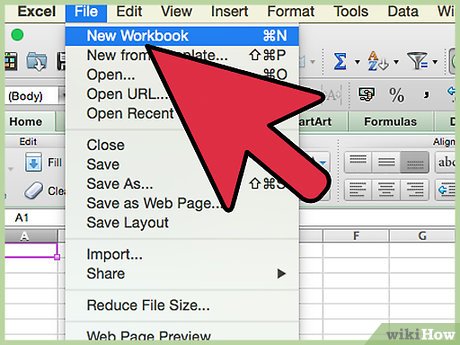
Start by opening a new Excel workbook and creating 3 worksheets: Tekeporter Data, Tekeporter Chart (unless you have Chart Wizard) and Tekeporter Saves, Save the workbook into a logical file.

For those who have already completed the article How to Make a Square of Spherical Helixes, it may well be possible to save loads of time by saving a copy of that file anew, and adapting this one's changes into it -- look especially at the value in B5, A5, a small change in the defined Name for N to N_ (and possibly p to p_), a new variable in H1 and H2 called NUM which has no dependent and doesn't do anything yet, as neither do MULTER1 and MULTER2 (left over from a sheet on which they were used to warp output for x and y) ... no, B5 looks to be the only serious change. Set B5 to "=25680/2/3/2/2/3/2"=178.3333, w/o quotes as usual. However, now would be a good opportunity to do Insert New Comment on all variables and formulas so there's a working copy of the original nearby. See also the formula in H1086 to see if there's a slight change there.

Set Preferences: Open Preferences in the Excel menu. Recommended Settings: Set General to R1C1 Off and Show the 10 Most Recent Documents; Edit - set all the Top options to checked except Automatically Convert Date System. Display number of decimal places = blank (for integers preferred), Preserve display of dates and set 30 for 21st century cutoff; View - show Formula Bar and Status Bar, hover for comments and all of Objects, Show gridlines and all boxes below that auto or checked; Chart - show chart names and data markers on hover. Leave rest unchecked for now; Calculation -- Automatically and calculate before save, max change .000,000,000,000,01 w/o commas if you do goal-seeking a lot and save external link values and use 1904 system; Error checking - check all; Save - save preview picture with new files and Save AutoRecover after 5 minutes; Ribbon -- all checked except Hide group titles and Developer.

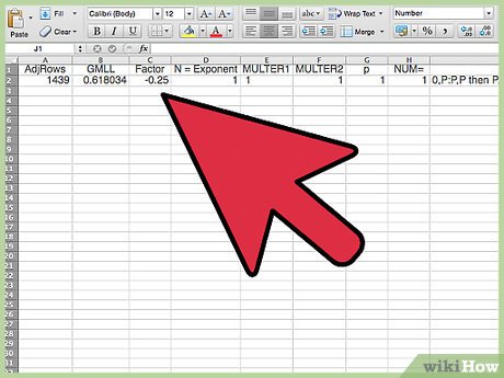
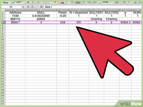
Enter the Defined Variable Names of Row 1 on the Data worksheet. A1: AdjRows; B1: GMLL (for 'Golden Mean Long Leg'); C1: Factor; D1: N_; E1: MULTER1; F1: MULTER2 G1: p; H1: NUM. Edit Go To cell range A1: H2 and Insert Create Names in Top Row. Then go back and change N to N = Exponent and NUM to NUM=. Click between the A and the 1 in the top left corner of the worksheet to select the entire worksheet and Format Cells Number Number Decimal Places 4, and Alignment Center.

Enter the Defined Name Variable Values and Formulas in Row 2. A2: 1439; B2: =0.618033988749895; C2: -.25; D2: 1; E2: 1; F2: 1, G2: 1; H2 1. Into I2 type the following left-aligned note, w/o quotes: "0,P:P,P then P,P to P,0 then P,0 to 0,0 then 0,0 to 0,P."

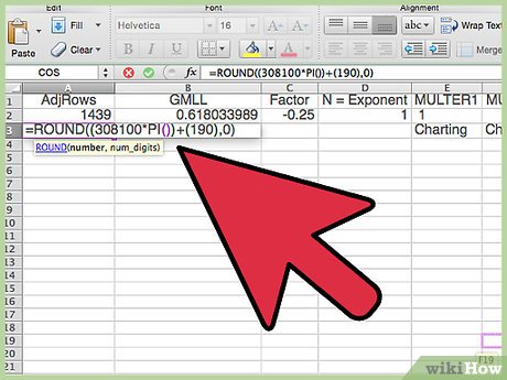
Enter a formula note into cell A3 w/o quotes: "=ROUND((308100*PI())+(190),0)"; enter another formula note into cell B3 w/o quotes: 25822. The A3 and B3 values are memos of values that work for A and B. Select cell E3 and type Charting, and do the same for F3.

Enter the Column Headings into Row 4. A4: Base t; B4: c; C4: Cos; D4 Sin; E4: x; F4: y; G4: Sides x; H4 Sides y. So when p=1, the I2 note forms a square of 4 sides of {x,y} pairs in columns G and H as follows: {0,1}:{1,1}, {1,1}:{1,0}, {1,0}:{0,0} and {0,0}:{0,1}. That's Top, Right, Bottom and Left Side.

Enter the Column Formulas.

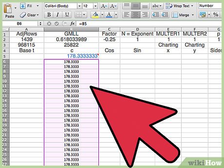
1. Enter into B5 the formula, w/o quotes, "=25680/2/3/2/2/3/2" (the result should be 178.3333). Insert New Comment and edit in "Original formula =25680/2/3/2/2/3/2 = 178.3333". Format cell Fill Light Blue, as its formula is distinct from the others in that column. Edit Go To cell range B6:B1445 and with B6 the active high-lighted cell, enter the formula, "=B5" and Edit Fill Down.
2. Enter into A5 the formula, w/o quotes, "=B5*12*PI()" and Insert New Comment and edit in "Original formula =B5*12*PI()". Format cell Fill Light Blue, as its formula is distinct from the others in that column. Insert Name Define Name top to cell $A$5. That's "top" is what is correct, w/o quotes.
3. Edit Go To cell range A6:A1445 and with A6 the active high-lighted cell, enter the formula, w/o quotes, "=(A5+(-top*2)/(AdjRows))" and Edit Fill Down. Do Insert New Comment and edit in "Original formula =(A5+(-top*2)/(AdjRows))". Done correctly, cell A1444 will be -6,723.0083, just the opposite of cell A5.
4. Edit Go To cell range C5:C1445 and with C5 the active high-lighted cell enter the formula w/o quotes, "=COS((ROW()-5)*PI()/180*Factor)". Now there are 1440 rows and 1440/360 = 4, so the Factor at -.25 is correct. Edit Fill Down and Insert New Comment and edit in "Original formula =COS((ROW()-5)*PI()/180*Factor) and 1440/360 = 4 so Factor = .25 is correct". Changing Factor to +.25 had no effect on the Chart. Cos(.25) = Cos(-.25) is why.
5. Edit Go To cell range D5:D1445 and with D5 the active high-lighted cell enter the formula w/o quotes, "=SIN((ROW()-5)*PI()/180*Factor)". Now there are 1440 rows and 1440/360 = 4, so the Factor at -.25 is correct. Edit Fill Down and Insert New Comment and edit in "Original formula =SIN((ROW()-5)*PI()/180*Factor) and 1440/360 = 4 so Factor = .25 is correct".
6. Edit Go To cell range E5:E1445 and with E5 the active high-lighted cell, enter the formula w/o quotes, "=((SIN(A5/(B5*2))*GMLL*COS(A5)*GMLL*(COS(A5/(B5*2)))*GMLL)+G5)^(N_-0)". Edit Fill Down and Insert New Comment and edit in "Original formula =((SIN(A5/(B5*2))*GMLL*COS(A5)*GMLL*(COS(A5/(B5*2)))*GMLL)+G5)^(N_-0)t". That is a zero, not an Oh, at the tail end -- it's for adjusting the exponent as between the Cosine and Sine. The addition of G5 instead of C5 will become apparent in a minute -- C5 makes a circle and G5 makes a square, Combinations are possible, so C5 was left in.
7. Edit Go To cell range F5:F1445 and with F5 the active high-lighted cell enter the formula w/o quotes, "=((SIN(A5/(B5*2))*GMLL*SIN(A5)*GMLL*(COS(A5/(B5*2)))*GMLL)+H5)^(N_-0)". Edit Fill Down and Insert New Comment and edit in "Original formula =((SIN(A5/(B5*2))*GMLL*SIN(A5)*GMLL*(COS(A5/(B5*2)))*GMLL)+H5)^(N_-0)". That is a zero, not an Oh, at the tail end -- it's for adjusting the exponent as between the Cosine and Sine. The addition of H5 instead of D5 will become apparent in a minute -- D5 makes a circle and H5 makes a square, Combinations are possible, so D5 was left in.

The sides of the square are the last thing to do before creating the chart. One side at a time will be done.

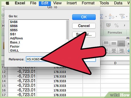
1. Side 1, the Top, from {0,1}:{1,1}. Edit Go To cell range H5:H365 and enter "=p" into cell H5 and Edit Fill Down. Insert New Comment and edit in "Original formula =p" w/o quotes. Select cell G5 and input 0 into it. Edit Go To the cell range G6:G365 and enter the formula w/o quotes, "=p/360+G5". Edit Fill Down. If Excel creates problems about p being a disallowed variable name, Insert Name Define Name p_ for cell G2, and substitute p_ for p wherever is mentioned p -- p works fine in the example sheet however, but it is a column name, so strictly speaking, it's probably disallowed now. I changed N to N_ for the same reason. Insert New Comment and edit in "Original formula =p/360+G5" (or p_/360+G5 -- whichever pertains). Edit Go To cell range G5:H365 and Format Cells Fill some nice color to differentiate it from the other sides.
2. Side 2, the Right, from {1,1}:{1,0}. Edit Go To cell range G366:G725 and enter "=p" into cell G366 and Edit Fill Down. Insert New Comment and edit in "Original formula =p" w/o quotes. Edit Go To cell range H366:H725 and input w/o quotes the formula "=-p/360+H365" into it. Insert New Comment and edit in "Original formula =-p/360+H365" (or -p_/360+H365 -- whichever pertains). Edit Go To cell range G366:H725 and Format Cells Fill some nice new color to differentiate it from the other sides.
3. Side 3, the Bottom, from {1,0}:{0,0}. Edit Go To cell range G726:G1085 and enter "=-p/360+G725" into cell G726 and Edit Fill Down. Insert New Comment and edit in "Original formula =-p/360+G725" w/o quotes. Edit Go To cell range H726:H1085 and input w/o quotes the formula "=0" into it. Insert New Comment and edit in "Original formula =0". Edit Fill Down. Edit Go To cell range G366:H725 and Format Cells Fill an entirely bright new color to differentiate the bottom from the other sides.
4. Side 4, the Left Side, from {0,0}:{0,1}. Edit Go To cell range G1086:G1445 and enter "=0" into cell G1086 and Edit Fill Down. Insert New Comment and edit in "Original formula =0" w/o quotes. Select cell H1086 and input w/o quotes the formula "=E5" and Insert Comment and edit in "Original Formula =E5". Edit Go To cell range H1087:H1445 and input w/o quotes the formula "=p/360+H1086" (or =p_/360+H1086) into it. Insert New Comment and edit in "Original formula =p/360+H1086". Edit Fill Down. Edit Go To cell range G1087:H1445 and Format Cells Fill a final differentiated color to make the final left side different from the other sides.

Create the Chart.

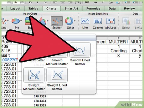
1. Edit Go To cell range E5:F1445 and use Chart Wizard to get a new Chart or use the Ribbon to select Chart, All. scroll down to Scatter, Smoothed Line Scatter and copy or cut and paste to the CHART worksheet the new chart. Double click in the chart and hover over the lower right corner until the double-headed arrow appears and pull it open in an expansion until a square is formed. This resizing business may require adjustment again -- leave it to the end of the chart formatting. .
2. Double-click on the vertical axis and set Scale as follows: Minimum: -.2, Maximum: 1.2; Major Unit 1.2; Minor Unit .2; Horizontal Axis is the only one checked and it crosses at 0.0. The chart is in Base 10. OK. Double-click on the horizontal axis and set Scale as follows: Minimum: -.2, Maximum: 1.2; Major Unit 1.2; Minor Unit .2; Vertical Axis is the only one checked and it crosses at 0.0. The chart is in Base 10. OK. With the Shift Key depressed, Copy Picture after clicking on the chart area, and activate the SAVES worksheet and Shift Key Paste Picture. One may wish to make some notes about the scale settings. Here is a picture of the chart w/o any axis or legend or grid lines or background, as one may wish to copy and stretch it immediately for some message or something -- those deletions are performed in Chart Layout and one can add a bottom reflection, or a shadow, or glow, etc. and put it in a frame or on a graphics work board, etc. -- many nice effects are possible:
   How to Create a Tekeporter Frame Image in Excel Picture 11