How to Rank Values in Excel from Highest to Lowest

To rank numbers in Excel, use RANK.EQ (or the older compatible RANK function). Set the final argument to 0 for highest-to-lowest ranking or 1 for lowest-to-highest ranking.

RANK function syntax

=RANK(number, ref, [order])

The arguments are:

• number: the value whose position you want to calculate.
• ref: the complete range of values being ranked.
• order: 0 or omitted ranks in descending order; any nonzero value ranks in ascending order.

Modern Excel versions also provide RANK.EQ and RANK.AVG. RANK.EQ gives tied values the same highest applicable rank, matching the behavior of RANK. RANK.AVG gives tied values the average of the positions they occupy.

Rank scores from highest to lowest

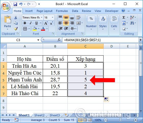
In the example, the scores are in cells B3:B7, and the ranking will be placed in the adjacent column.

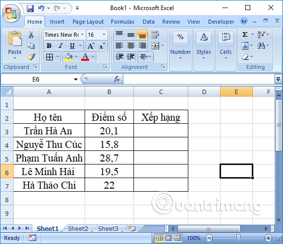
1. Select the first result cell in the Ranking column.

2. Enter:

   =RANK(B3,$B$3:$B$7,0)

3. Press Enter, then drag the fill handle down to copy the formula to the remaining rows.

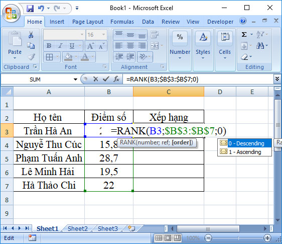
Here, B3 changes to B4, B5, and so on as the formula is copied. The dollar signs keep $B$3:$B$7 fixed so every row is compared with the same complete range.

A result of 1 identifies the highest score. In the sample, the first student's score returns rank 3.

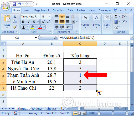
Rank values from lowest to highest

Use 1 as the order argument when the smallest number should be rank 1:

=RANK(B3,$B$3:$B$7,1)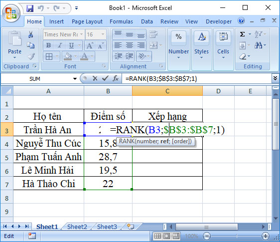

Copy the formula down the column. The lowest score now receives rank 1, and the highest receives the largest rank number.

How Excel handles ties

With RANK or RANK.EQ, equal values receive the same rank and the next position is skipped. For example, if two values tie for second place, the following value is ranked fourth.

If you want tied values to receive the average of their occupied positions, use:

=RANK.AVG(B3,$B$3:$B$7,0)

Common mistakes

• Reversing the order argument: 0 means descending, not ascending.
• Forgetting absolute references: without dollar signs, the comparison range moves when the formula is copied.
• Leaving text in the score range: verify that the values are stored as numbers.
• Expecting unique positions: standard ranking functions intentionally return ties.