How to use the TREND function in Excel

You can calculate and visualize trends in Excel using the TREND function . Doing so will give you insights into your data and make it easier to make forecasts. 

How to use the TREND function in Excel Picture 1

What is Trend Line?

A trend line is a straight line that shows whether data is increasing or decreasing over time. It is often applied to time series, where you can track values ​​over specific time periods.

A trendline serves as a visual representation of a trend, showing the general direction of your data. It rarely fits all the values ​​in a series perfectly unless they are already aligned in a straight line. Instead, it is the best possible approximation, giving you a clear sense of the overall movement.

One of the most practical uses of a trendline is prediction. By extending a trend, you can predict future values. This is where the slope of the line becomes essential—it shows the speed and direction of the trend. However, calculating a trend manually is tedious and, of course, error-prone. That's where Excel's TREND function comes in handy.

What is the TREND function in Excel?

TREND is a statistical function that uses your known data (X and Y) to create a trend line and predict future values. Its syntax is simple:

=TREND([known_Ys], [known_Xs], [new_Xs], [const])

The first two arguments, known_Ys and known_Xs, are the data you already have. new_Xs is the data you want to predict and calculate the trend for. The const argument determines whether to include the intercept value (b) in the trendline equation (y = ax + b). If set to TRUE or omitted, Excel calculates a intercept value; if set to FALSE, Excel assumes no intercept value.

How to use the TREND function in Excel

To better understand TREND, let's look at an example. Let's say you have eight known Y values ​​(1 through 8) and their corresponding X values ​​(also 1 through 8). You're missing values ​​for times 9 and 10 and you want Excel to project them.

How to use the TREND function in Excel Picture 2

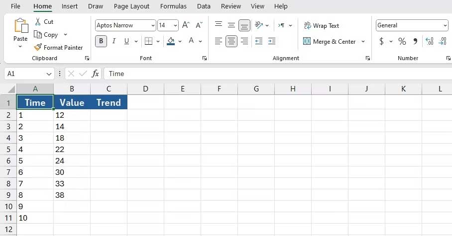
First, click on the cell where you want the new Ys to appear (C2 in this example). Then, enter the formula below in the formula bar:

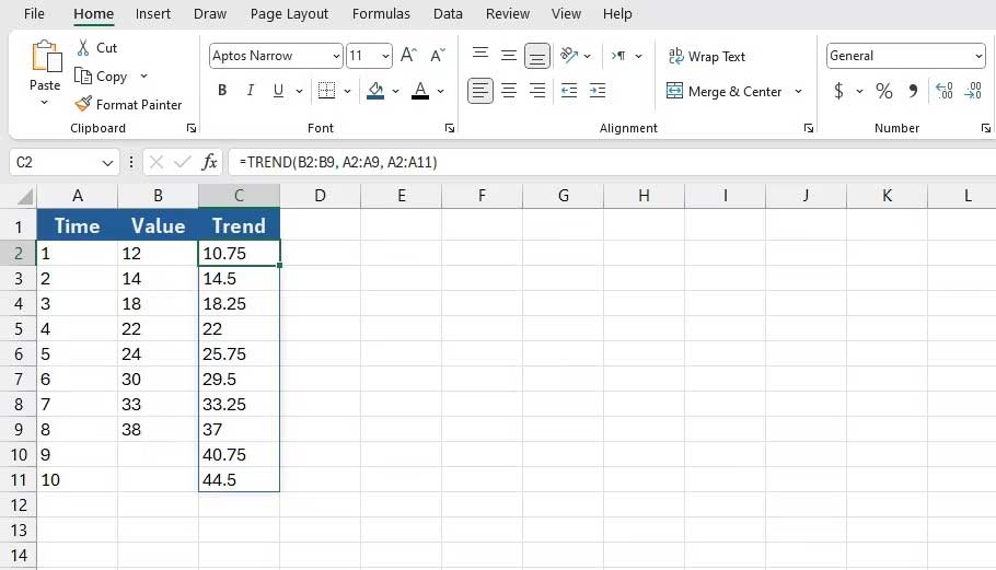
=TREND(B2:B9, A2:A9, A2:A11)

This formula calls the TREND function and plugs in cells B2:B9 as the known Ys . Then it plugs in A2:A9 as the known Xs . Finally, the formula tells TREND that A2:A11 will be the new Ys. These new Ys are calculated outside the trendline.

When you press Enter , Excel fills the cells with the trend values. Observe how the predicted Ys in the trend, although linear, are close to the known Ys.

How to use the TREND function in Excel Picture 3

Above is how to use the TREND function in Microsoft Excel . Hope the article is useful to you.

Kareem Winters

Update 11 September 2024